| LEVEL 1 BREAKOUT | LEVEL 2 BREAKOUT | ||||||||
|---|---|---|---|---|---|---|---|---|---|
| TOTAL MILES: | 1000 | ||||||||
| Terrain Type | Percent | Miles | Speed | Surface¹ | Percent | Miles | Speed | ||
| Max | Avg | Max | Avg | ||||||
| PRIMARY ROAD | 70% | 700 | 55 | 35 | Paved | 100% | 700 | 55 | 35 |
| 100% | 700 | ||||||||
| SECONDARY ROAD | 20% | 200 | 40 | 22 | Secondary Road | 60% | 120 | 40 | 25 |
| Gravel Road | 23% | 46 | 45 | 22 | |||||
| Belgian Block | 10% | 20 | 25 | 15 | |||||
| Embedded Rock | 1% | 2 | 10 | 7 | |||||
| Radial Washboard | 3% | 6 | 15 | 9 | |||||
| 2" Washboard | 3% | 6 | 10 | 7 | |||||
| 100% | 200 | ||||||||
| * Off Road | 10% | 100 | 25 | 14 | Cross Country | 85% | 85 | 25 | 16.3 |
| * A combination of trails and cross country | Embedded Rock | 5% | 5 | 10 | 7 | ||||
| Radial Washboard | 5% | 5 | 15 | 9 | |||||
| 2" Washboard | 5% | 5 | 10 | 7 | |||||
| 100% | 100 | ||||||||
| LEVEL 1 | This information should be provided by the program manager and is required before LVTS development can begin. This information can sometimes be found in the LCEP or other system documentation. | ||||||||
| LEVEL 2 | This breakout has a significant impact on the test durations of the final LVTS and should therefore be given serious consideration. This information, too, should be provided but is seldom available. Development cannot begin without this breakout. Often the analyst is forced to recommend a breakout for the concurrence of user. | ||||||||
MIL-STD-810H METHOD 514.8, ANNEX F
514.8F -II: Selection of Alpha for Beta Distribution
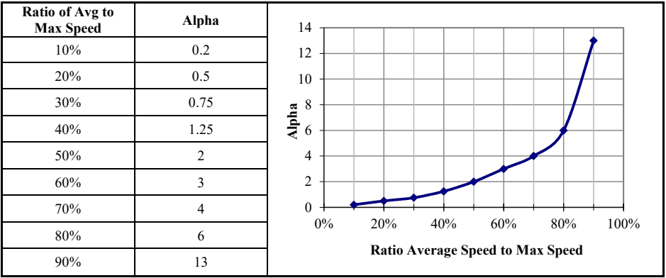
Figure description:
Legend
- Alpha — color: Dark blue; symbol: Line with diamond markers
| Ratio of Avg to Max Speed | Alpha |
|---|---|
| 10% | 0.2 |
| 20% | 0.5 |
| 30% | 0.75 |
| 40% | 1.25 |
| 50% | 2 |
| 60% | 3 |
| 70% | 4 |
| 80% | 6 |
| 90% | 13 |
Notes: The image displays a data table and its corresponding line graph showing the relationship between the ratio of average speed to maximum speed and the parameter Alpha. The graph shows an exponential-like increase in Alpha as the ratio approaches 100%.
MIL-STD-810H
METHOD 514.8, ANNEX F
| BETA DISTRIBUTION INPUTS | |
|---|---|
| SURFACE | Paved Road |
| MIN SPEED OF DATA SET | 5 |
| MAX SPEED OF DATA SET | 55 |
| AVG SPEED FROM SCENARIO | 35 |
| SPEED INCREMENT OF DATA SET | 5 |
| TOTAL MILES FROM SCENARIO | 700.00 |
| TOTAL HOURS | 20.000 |
| Ratio Avg/Max Speed | 64% |
| CALCULATED RESULTS | |
|---|---|
| Dist Min Speed | 0 |
| Dist Max Speed | 57.5 |
| ALPHA | 3.40 |
| BETA | 2.19 |
| Average Speed | 35.00 |
| Total Miles | 699.982 |
| Total Hours | 20.000 |
| Error | 0.00% |
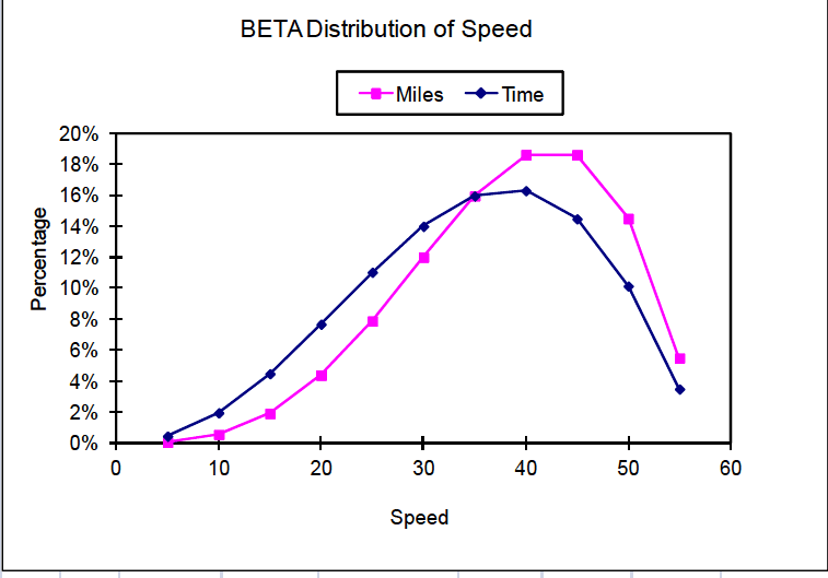
Figure description:
BETA Distribution of Speed
BETA Distribution of Speed
Legend
- Miles — color: magenta; symbol: Solid line with square marker
- Time — color: dark blue; symbol: Solid line with diamond marker
| Speed | Miles (Percentage) | Time (Percentage) |
|---|---|---|
| 5 | 0.1% | 0.4% |
| 10 | 0.5% | 2.0% |
| 15 | 1.9% | 4.5% |
| 20 | 4.3% | 7.6% |
| 25 | 7.8% | 11.0% |
| 30 | 12.0% | 14.0% |
| 35 | 15.9% | 16.0% |
| 40 | 18.6% | 16.3% |
| 45 | 18.6% | 14.5% |
| 50 | 14.5% | 10.1% |
| 55 | 5.5% | 3.5% |
| BETA DISTRIBUTION OF SPEED | ||||||||
|---|---|---|---|---|---|---|---|---|
| Repr | Start | End | Range | Percentage | Time | Percentage | ||
| Speed | Speed | Speed | Avg | Time | in Hours | in Min | Miles | Miles |
| n/a | 0 | 2.5 | 1.25 | 0.012% | 0.002 | 0.15 | 0.0031 | 0.00% |
| 5 | 2.5 | 7.5 | 5 | 0.458% | 0.092 | 5.50 | 0.46 | 0.07% |
| 10 | 7.5 | 12.5 | 10 | 1.966% | 0.393 | 23.59 | 3.93 | 0.56% |
| 15 | 12.5 | 17.5 | 15 | 4.487% | 0.897 | 53.84 | 13.46 | 1.92% |
| 20 | 17.5 | 22.5 | 20 | 7.673% | 1.535 | 92.08 | 30.69 | 4.38% |
| 25 | 22.5 | 27.5 | 25 | 11.035% | 2.207 | 132.42 | 55.18 | 7.88% |
| 30 | 27.5 | 32.5 | 30 | 13.999% | 2.800 | 167.99 | 84.00 | 12.00% |
| 35 | 32.5 | 37.5 | 35 | 15.955% | 3.191 | 191.46 | 111.68 | 15.95% |
| 40 | 37.5 | 42.5 | 40 | 16.295% | 3.259 | 195.54 | 130.36 | 18.62% |
| 45 | 42.5 | 47.5 | 45 | 14.478% | 2.896 | 173.74 | 130.31 | 18.62% |
| 50 | 47.5 | 52.5 | 50 | 10.142% | 2.028 | 121.71 | 101.42 | 14.49% |
| 55 | 52.5 | 57.5 | 55 | 3.499% | 0.700 | 41.99 | 38.49 | 5.50% |
| TOTAL | 100.0% | 20.000 | 1200.00 | 699.982 | 100.0% | |||
| TOTAL USED | 100.0% | 19.998 | 1199.85 | 699.979 | 100.0% | |||
Figure 514.8F-1. Sample beta distribution (wheeled vehicle).
The Beta distribution calculations are performed in the “BETA DISTRIBUTION OF SPEED” table of Figure 514.8F-1. A description of the fields follows.
- a. Repr Speed - The representative speed for this entry. This is the speed for which vibration data were acquired.
- b. Start Speed – The beginning of the speed range for this entry.
- c. End Speed – The ending of the speed range for this entry.
- d. Range Average – The average of the speed range for this entry. This number should be equal to the representative speed for the entry.
- e. Percentage Time – This is the actual Beta distribution as a percentage of the total drive time. This column, along with the Percentage Miles column, is plotted on the graph of Figure 514.8F-1.
- f. Time in Hours – The time in hours represented by this data entry, calculated by multiplying the total hours by the percentages of the previous column. The total hours is calculated from the total miles and the average speed.
- g. Time in Min. – The time in minutes represented by this data entry. This is the final output of the Beta distribution and is passed forward to the VSD process.
- h. Miles – The miles represented by this data entry, calculated by multiplying the Time in Hours by the Range Average.
- i. Percentage Miles – The percentage of the total miles represented by this entry. This column, along with the Percentage Time column, is plotted on the graph of Figure 514.8F-1.
Note that the widths (in units of speed) of each speed range in the table of Figure 514.8F-1 are equal to the speed increment for which data was acquired and are centered around the acquired speeds. This results in two slight inconsistencies at the endpoints of the Beta distribution. First, the percentage of the miles at very low speeds (below 2.5 mph in this example) is not included in the VSD process. It is expected that the vibration at these speeds will be quite low and have no effect on the resultant LVTS, even if included. Second, the maximum speed of the Beta distribution is one-half speed increment higher than the highest speed for which data was acquired. This too should have little effect on the VSD process since very little time is spent at this speed.
The endpoints of the Beta distribution technique are treated slightly different for NBROR or SOR LVTS. In those cases, the endpoints for Beta distribution are set to exactly the minimum and maximum speeds acquired. If the example presented here were for a tracked vehicle the range of the first entry would be from 5 to 7.5 mph instead of 2.5 to 7.5 mph. Likewise, the last entry would be from 42.5 to 45 mph instead of 42.5 to 47.5 mph. For a tracked vehicle the narrowband random sweeps dominate the fatigue exposure represented by an LVTS. The same is true for the swept sine LVTS. Therefore, more emphasis is placed on the sweep ranges when calculating the Beta distribution. The sweep ranges are bound by the frequencies associated with the minimum and maximum speeds acquired, and the Beta distribution ranges are selected to account for that. Note that the speed ranges of the endpoints are then one-half as wide as the intermediate points. This is accounted for in the VSD process when calculating the actual run time represented by each speed event. The run times of the first and last speeds are set to one half of the intermediate speeds. Note also that during testing on the shaker, the swept narrow bands are in the range of the endpoint speeds for one-half the time of the other speeds.
514.8F -C.I. Test Course Lengths, Speeds and Exposure Times
| Test Course | |||
|---|---|---|---|
| Length, m (ft) | Nominal Speed, km/hr (mph) | Exposure Time, sec | |
| Belgian Block | 1200 (3940) | 32.2 (20) | 134 |
| Two-Inch Washboard | 250 (822) | 16.2 (10) | 56 |
| Radial Washboard | 74 (243) | 24.1 (15) | 11 |
| Three Inch Spaced Bump | 233 (764) | 32.2 (20) | 26 |
| Total | 1757 (5769) | 227 |
The exposure times can be used with equation C.1 and the appropriate test course ASDs to produce a fatigue damage spectrum for each test course. Using the same set of typical wheeled vehicle data as before, the fatigue spectra are shown in Figure 514.8F-C.1. For this example, was chosen to be 0.05 (5-percent critical damping) and the exponent was substituted for , and was assigned a value of 7.5 .
MIL-STD-810H METHOD 514.8, ANNEX F, APPENDIX C
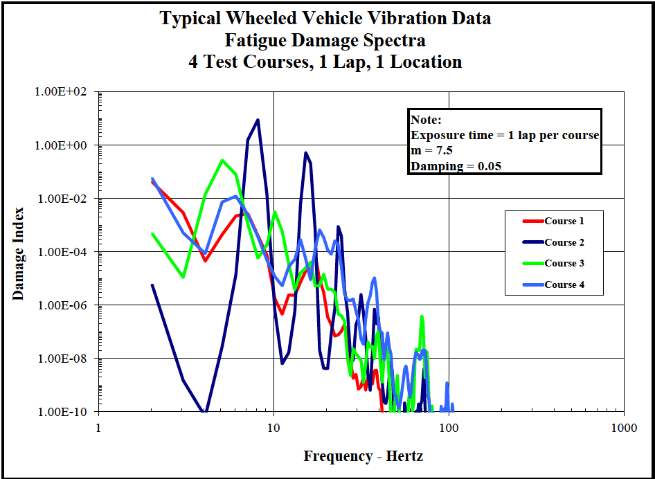
Figure description:
Typical Wheeled Vehicle Vibration Data 4 Test Courses, 1 Lap, 1 Location
Fatigue Damage Spectra
Legend
- Course 1 — color: red; symbol: Solid line
- Course 2 — color: dark blue; symbol: Solid line
- Course 3 — color: green; symbol: Solid line
- Course 4 — color: light blue; symbol: Solid line
Annotations
- Exposure time = 1 lap per course (text_label - position: x = 40, y = 1.00E+01)
- m = 7.5 (text_label - position: x = 40, y = 1.00E+00)
- Damping = 0.05 (text_label - position: x = 40, y = 1.00E-01)
| Frequency - Hertz | Course 1 | Course 2 | Course 3 | Course 4 |
|---|---|---|---|---|
| 2 | 5.00E-02 | 6.00E-06 | 5.00E-04 | 6.00E-02 |
| 3 | 5.00E-03 | 2.00E-08 | 1.00E-05 | 5.00E-04 |
| 4 | 4.00E-05 | 1.00E-10 | 2.00E-03 | 2.00E-04 |
| 5 | 5.00E-04 | 1.00E-08 | 3.00E-01 | 8.00E-03 |
| 6 | 1.00E-03 | 5.00E-06 | 1.00E-01 | 1.00E-02 |
| 7 | 2.00E-03 | 2.00E+00 | 2.00E-04 | 1.00E-02 |
| 8 | 3.00E-03 | 1.00E+01 | 6.00E-05 | 3.00E-03 |
| 9 | 1.00E-03 | 3.00E-01 | 1.00E-04 | 5.00E-04 |
| 10 | 1.00E-04 | 2.00E-04 | 3.00E-03 | 1.00E-05 |
| 15 | 2.00E-06 | 5.00E-01 | 1.00E-05 | 3.00E-04 |
| 20 | 2.00E-07 | 5.00E-09 | 1.00E-05 | 1.00E-04 |
| 25 | 1.00E-07 | 1.00E-03 | 3.00E-07 | 3.00E-04 |
| 30 | 1.00E-09 | 1.00E-06 | 2.00E-08 | 1.00E-07 |
| 40 | 1.00E-10 | 1.00E-08 | 1.00E-07 | 1.00E-05 |
| 50 | null | 1.00E-10 | 1.00E-09 | 5.00E-09 |
| 70 | null | 2.00E-09 | 4.00E-07 | 2.00E-08 |
| 100 | null | 1.00E-10 | 1.00E-10 | 1.00E-09 |
Notes: The chart uses logarithmic scales for both the X-axis (Frequency in Hertz and the Y-axis (Damage Index. The data values in the markdown table are estimates derived from the plot. Exposure time, m factor, and damping ratio are specified in a note within the chart area.))
Figure 514.8F-C.1. Fatigue damage spectra for specific test courses.
The cumulative fatigue damage spectrum (equation C.2) is shown by the lavender line in Figure 514.8F-C.2 and represents a fatigue damage index derived from a complete lap of the four specified test courses.
MIL-STD-810H METHOD 514.8, ANNEX F, APPENDIX C
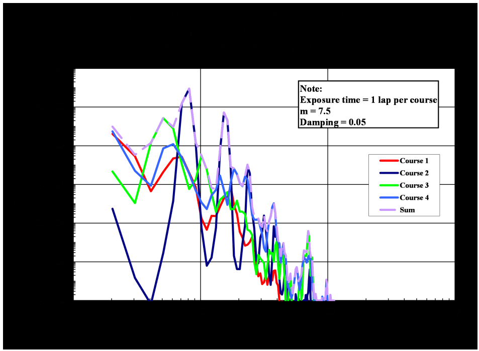
Figure description:
Typical Wheeled Vehicle Vibration Data 4 Test Courses, 1 Lap, 1 location
Fatigue Damage Spectra
Legend
- Course 1 — color: red; symbol: Solid line
- Course 2 — color: dark blue; symbol: Solid line
- Course 3 — color: bright green; symbol: Solid line
- Course 4 — color: light blue; symbol: Solid line
- Sum — color: light purple; symbol: Solid line
Annotations
- Note: Exposure time = 1 lap per course, m = 7.5, Damping = 0.05 (text_label - position: top right)
| Frequency (Hertz) | Course 1 | Course 2 | Course 3 | Course 4 | Sum |
|---|---|---|---|---|---|
| 2 | 5.00E-02 | 6.00E-06 | 5.00E-04 | 5.00E-02 | 1.00E-01 |
| 3 | 1.00E-02 | 2.00E-09 | 1.00E-05 | 5.00E-03 | 1.50E-02 |
| 4 | 5.00E-05 | 1.00E-10 | 2.00E-02 | 1.00E-04 | 2.00E-02 |
| 5 | 1.00E-03 | 3.00E-08 | 2.00E-01 | 8.00E-03 | 2.10E-01 |
| 6 | 2.00E-03 | 1.00E-06 | 8.00E-02 | 1.20E-02 | 9.50E-02 |
| 7 | 3.00E-03 | 1.00E-01 | 1.00E-04 | 5.00E-03 | 1.10E-01 |
| 8 | 1.00E-03 | 8.00E+00 | 5.00E-04 | 2.00E-03 | 8.00E+00 |
| 9 | 5.00E-04 | 1.00E+00 | 1.00E-04 | 5.00E-04 | 1.00E+00 |
| 10 | 1.00E-05 | 1.00E-04 | 2.00E-03 | 1.00E-04 | 2.20E-03 |
| 12 | 1.00E-05 | 2.00E-03 | 5.00E-04 | 2.00E-04 | 2.70E-03 |
| 15 | 5.00E-05 | 1.00E+00 | 1.00E-04 | 3.00E-04 | 1.00E+00 |
| 20 | 1.00E-05 | 1.00E-05 | 1.00E-05 | 6.00E-04 | 6.30E-04 |
| 25 | 2.00E-07 | 5.00E-04 | 2.00E-06 | 2.00E-04 | 7.00E-04 |
| 30 | 1.00E-08 | 2.00E-06 | 1.00E-07 | 2.00E-06 | 4.10E-06 |
| 40 | 1.00E-09 | 1.00E-05 | 1.00E-07 | 1.00E-05 | 2.00E-05 |
| 50 | 1.00E-10 | 2.00E-09 | 5.00E-10 | 2.00E-09 | 5.00E-09 |
| 60 | 1.00E-10 | 1.00E-09 | 1.00E-09 | 2.50E-08 | 2.70E-08 |
| 70 | 1.00E-10 | 4.00E-07 | 3.00E-07 | 1.50E-08 | 7.20E-07 |
| 80 | 1.00E-10 | 1.00E-10 | 1.00E-10 | 1.00E-10 | 1.00E-10 |
| 100 | 1.00E-10 | 1.00E-10 | 1.00E-10 | 1.00E-10 | 1.00E-10 |
Notes: The data represents a Fatigue Damage Spectra (FDS for four test courses. Both axes are on a logarithmic scale. The Y-axis represents Damage index and the X-axis represents Frequency in Hertz.)
Figure 514.8F-C.2. Cumulative fatigue damage spectrum (lavender line).
The same process was performed for 2 measurement locations independently using cumulative data for 3 laps. The cumulative spectra for each location were then averaged and enveloped for comparison and are shown in Figure 514.8F-C.3.
MIL-STD-810H METHOD 514.8, ANNEX F, APPENDIX C
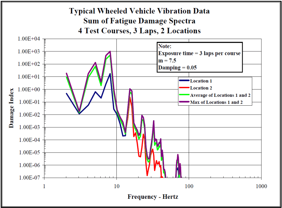
Figure description:
Typical Wheeled Vehicle Vibration Data Sum of Fatigue Damage Spectra 4 Test Courses, 3 Laps, 2 Locations
Sum of Fatigue Damage Spectra
Legend
- Location 1 — color: dark blue; symbol: solid line
- Location 2 — color: red; symbol: solid line
- Average of Locations 1 and 2 — color: light green; symbol: solid line
- Max of Locations 1 and 2 — color: purple; symbol: solid line
Annotations
- Note: Exposure time = 3 laps per course m = 7.5 Damping = 0.05 (text_label - position: top right of plot area
| Frequency - Hertz | Location 1 | Location 2 | Average of Locations 1 and 2 | Max of Locations 1 and 2 |
|---|---|---|---|---|
| 2.0 | 4.70E-01 | 1.80E+01 | 9.24E+00 | 1.80E+01 |
| 3.0 | 1.10E-02 | 1.50E-02 | 1.30E-02 | 1.50E-02 |
| 4.0 | 5.50E-02 | 1.60E+01 | 8.03E+00 | 1.60E+01 |
| 5.0 | 6.50E-01 | 1.40E+02 | 7.03E+01 | 1.40E+02 |
| 6.0 | 2.00E-01 | 3.50E+00 | 1.85E+00 | 3.50E+00 |
| 8.0 | 1.80E+01 | 9.50E+02 | 4.84E+02 | 9.50E+02 |
| 10.0 | 2.50E-02 | 5.50E-02 | 4.00E-02 | 5.50E-02 |
| 12.0 | 2.10E-04 | 8.00E-04 | 5.05E-04 | 8.00E-04 |
| 14.0 | 5.00E-01 | 1.20E-01 | 3.10E-01 | 5.00E-01 |
| 15.0 | 1.10E+00 | 2.50E-01 | 6.75E-01 | 1.10E+00 |
| 17.0 | 1.00E-03 | 1.50E-04 | 5.75E-04 | 1.00E-03 |
| 20.0 | 2.00E-04 | 5.00E-06 | 1.03E-04 | 2.00E-04 |
| 23.0 | 9.00E-03 | 3.00E-04 | 4.65E-03 | 9.00E-03 |
| 27.0 | 1.00E-06 | 1.40E-07 | 5.70E-07 | 1.00E-06 |
| 30.0 | 2.00E-05 | 1.50E-06 | 1.08E-05 | 2.00E-05 |
| 33.0 | 3.30E-03 | 2.00E-05 | 1.66E-03 | 3.30E-03 |
| 37.0 | 1.00E-04 | 1.50E-06 | 5.08E-05 | 1.00E-04 |
| 40.0 | 1.20E-04 | 2.10E-06 | 6.11E-05 | 1.20E-04 |
| 45.0 | 5.00E-07 | null | 2.50E-07 | 5.00E-07 |
| 75.0 | 7.00E-06 | 2.00E-07 | 3.60E-06 | 7.00E-06 |
| 85.0 | 1.00E-07 | null | null | 1.00E-07 |
Notes: The Y-axis (Damage Index and X-axis (Frequency - Hertz are both on logarithmic scales. Data points were estimated based on the log-log grid provided.))
Figure 514.8F-C.3. Cumulative fatigue spectra from locations 1 and 2.
If an overall exposure time is selected, equation C.1 can be reworked to provide an ASD level based on the fatigue spectrum computed from Equation C.2.
C.3
| where: | |
|---|---|
| DP(fn) = | Cumulative damage index as a function of system natural frequency |
| fn = | System natural frequency (variable), Hz |
| T = | Total exposure time in environment, seconds |
| G(fn) = | Equivalent ASD for a given DP(fn), T, g2/Hz |
| ζ = | Damping ratio of system at dominant natural frequency expressed as a decimal |
| b = | Fatigue curve slope value when computed as a linear fit in log-log domain. |
MIL-STD-810H METHOD 514.8, ANNEX F, APPENDIX C
Using an exposure time equal to 3 times the total value listed in Table 514.8F-C.I (to account for 3 laps) and the fatigue damage spectra (average and max) shown in Figure 514.8F-C.3, an equivalent representative ASD was calculated from equation C.3. The spectra derived from the average and maximum fatigue damage spectra are shown in Figure 514.8F-C.4. For this data set, the fatigue damage spectra for locations 1 and 2 were nearly the same producing an average spectrum that is about the same as the enveloped spectrum. The enveloped or maximum spectrum is compared to the resultant spectrum computed from the statistical process and from a spectrum derived from the envelope of all original spectra and is shown in Figure 514.8F-C.5.
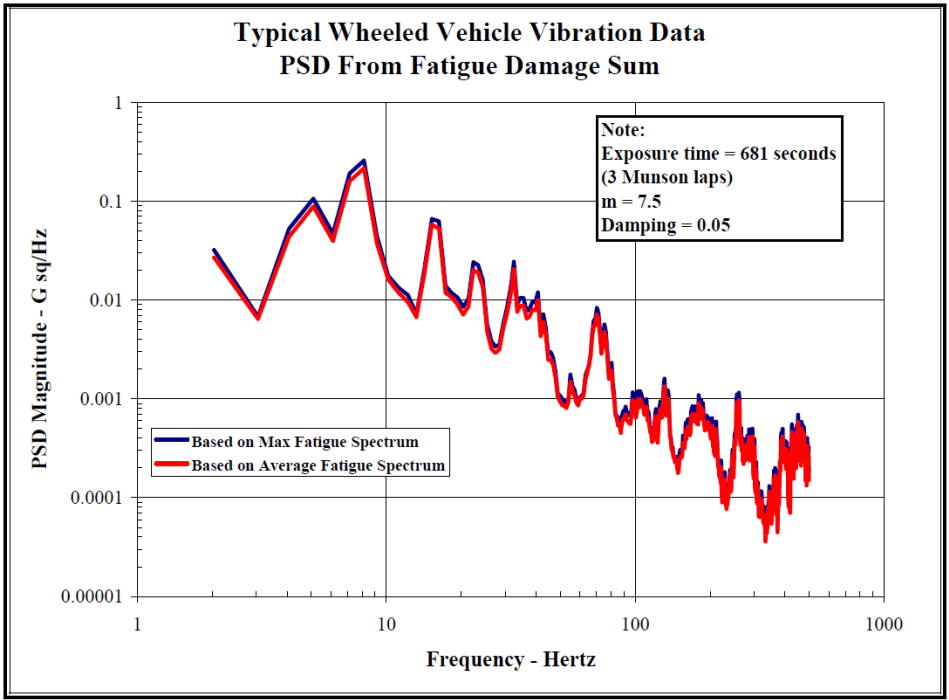
Figure description:
Typical Wheeled Vehicle Vibration Data PSD From Fatigue Damage Sum
PSD From Fatigue Damage Sum
Legend
- Based on Max Fatigue Spectrum — color: blue; symbol: Solid line
- Based on Average Fatigue Spectrum — color: red; symbol: Solid line
Annotations
- Note: Exposure time = 681 seconds (3 Munson laps m = 7.5 Damping = 0.05 (text_label - position: top right of graph area))
| Frequency - Hertz | Based on Max Fatigue Spectrum (G sq/Hz) | Based on Average Fatigue Spectrum (G sq/Hz) |
|---|---|---|
| 2.0 | 0.033 | 0.027 |
| 3.0 | 0.007 | 0.0065 |
| 4.0 | 0.054 | 0.048 |
| 5.0 | 0.107 | 0.092 |
| 6.0 | 0.046 | 0.039 |
| 7.1 | 0.198 | 0.176 |
| 8.0 | 0.264 | 0.233 |
| 9.5 | 0.036 | 0.028 |
| 10.3 | 0.017 | 0.015 |
| 13.5 | 0.009 | 0.0068 |
| 15.3 | 0.068 | 0.061 |
| 17.5 | 0.013 | 0.011 |
| 20.3 | 0.0089 | 0.0074 |
| 23.0 | 0.024 | 0.021 |
| 27.5 | 0.0035 | 0.0031 |
| 35.0 | 0.025 | 0.022 |
| 40.5 | 0.0071 | 0.0063 |
| 50.5 | 0.012 | 0.0094 |
| 62.0 | 0.0011 | 0.00086 |
| 71.0 | 0.0083 | 0.0071 |
| 95.0 | 0.0011 | 0.00092 |
| 104.0 | 0.0012 | 0.0011 |
| 130.0 | 0.0016 | 0.0013 |
| 160.0 | 0.00042 | 0.00033 |
| 185.0 | 0.0010 | 0.00085 |
| 235.0 | 0.00018 | 0.00014 |
| 265.0 | 0.0011 | 0.00095 |
| 320.0 | 0.000078 | 0.000057 |
| 420.0 | 0.00068 | 0.00052 |
| 500.0 | 0.00042 | 0.00031 |
Notes: The chart uses a logarithmic scale for both axes. Frequency ranges from 1 to 1000 Hertz, and PSD Magnitude ranges from 0.00001 to 1 G sq/Hz.
Figure 514.8F-C.4. Combined vibration power spectra developed from average and maximum fatigue damage Spectra.
MIL-STD-810H METHOD 514.8, ANNEX F, APPENDIX C
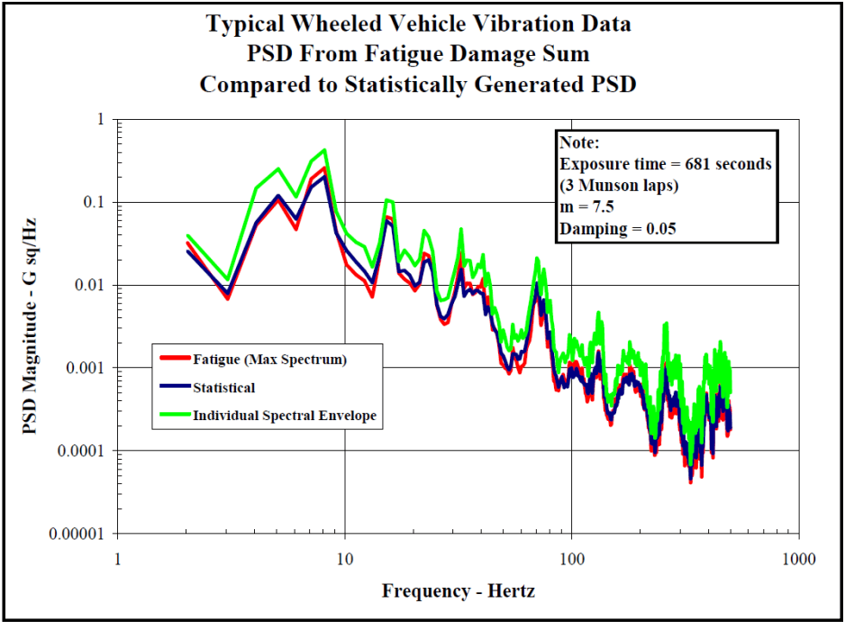
Figure description:
Typical Wheeled Vehicle Vibration Data PSD From Fatigue Damage Sum Compared to Statistically Generated PSD
Legend
- Fatigue (Max Spectrum — color: red; symbol: Solid line
- Statistical — color: dark blue; symbol: Solid line
- Individual Spectral Envelope — color: green; symbol: Solid line
Annotations
- Note: Exposure time = 681 seconds (3 Munson laps, m = 7.5, Damping = 0.05 (text_label - position: top right))
| Frequency - Hertz | Fatigue (Max Spectrum - PSD Magnitude (G sq/Hz)) | Statistical - PSD Magnitude (G sq/Hz) | Individual Spectral Envelope - PSD Magnitude (G sq/Hz) |
|---|---|---|---|
| 2.0 | 0.03 | 0.025 | 0.04 |
| 3.0 | 0.007 | 0.008 | 0.012 |
| 4.0 | 0.05 | 0.045 | 0.14 |
| 5.0 | 0.11 | 0.11 | 0.25 |
| 6.5 | 0.05 | 0.06 | 0.11 |
| 7.5 | 0.15 | 0.13 | 0.3 |
| 8.5 | 0.26 | 0.21 | 0.42 |
| 10.0 | 0.017 | 0.025 | 0.043 |
| 15.0 | 0.07 | 0.065 | 0.105 |
| 18.0 | 0.013 | 0.015 | 0.026 |
| 23.0 | 0.025 | 0.02 | 0.047 |
| 30.0 | 0.0035 | 0.004 | 0.006 |
| 37.0 | 0.02 | 0.009 | 0.048 |
| 55.0 | 0.001 | 0.0009 | 0.002 |
| 70.0 | 0.007 | 0.006 | 0.021 |
| 100.0 | 0.0006 | 0.0007 | 0.0023 |
| 135.0 | 0.001 | 0.001 | 0.0048 |
| 170.0 | 0.00025 | 0.0003 | 0.0012 |
| 210.0 | 0.0008 | 0.0006 | 0.0018 |
| 250.0 | 0.0001 | 0.00015 | 0.00035 |
| 290.0 | 0.0003 | 0.0002 | 0.0035 |
| 350.0 | 0.00004 | 0.00006 | 0.00012 |
| 420.0 | 0.0003 | 0.00025 | 0.0015 |
| 500.0 | 0.0002 | 0.00015 | 0.0008 |
Notes: The chart is a log-log plot representing PSD Magnitude vs. Frequency for wheeled vehicle vibration data.
Figure 514.8F-C.5. Comparison of combined vibration power spectrum developed from the fatigue damage
spectrum, from the statistical process and from an envelope process.
The three processes (fatigue spectrum, statistical and envelope) produce specifications that are roughly the same shape. The specification derived from the fatigue damage spectrum technique has lower levels than those produced by the envelope process and nearly the same (but generally lower) levels than those produced by the technique developed in Appendix B. The statistical technique contains an implied assumption that each environment has the same exposure time and weights the spectral values toward the most severe spectrum due to the inclusion of spectral variance (the addition of a standard deviation) in the process. Therefore, it is likely that the statistical process will produce higher levels than the fatigue damage process unless the most severe spectra also have the longest exposure times.
The process was repeated for an exponent value of m = 5 as a comparison. A comparison of the fatigue damage spectra (maximum) for the two exponents is shown in Figure 514.8F-C.6, and a comparison of the vibration power spectra developed from each exponent is presented in Figure 514.8F-C.7.
MIL-STD-810H METHOD 514.8, ANNEX F, APPENDIX C
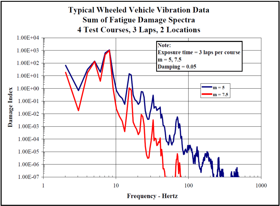
Figure description:
Typical Wheeled Vehicle Vibration Data Sum of Fatigue Damage Spectra, 4 Test Courses, 3 Laps, 2 Locations
Sum of Fatigue Damage Spectra
Legend
- m = 5 — color: blue; symbol: Solid line
- m = 7.5 — color: red; symbol: Solid line
Annotations
- Note: Exposure time = 3 laps per course, m = 5, 7.5, Damping = 0.05 (text_label - position: top right of plot area)
| Frequency - Hertz | m = 5 | m = 7.5 |
|---|---|---|
| 2.0 | 6.50E+01 | 1.80E+01 |
| 3.0 | 7.00E-01 | 1.80E-02 |
| 5.0 | 1.40E+02 | 1.10E+02 |
| 6.5 | 2.00E+01 | 4.00E+00 |
| 8.0 | 1.00E+03 | 1.10E+03 |
| 10.0 | 5.00E-01 | 2.00E-02 |
| 13.0 | 6.00E-02 | 4.00E-04 |
| 15.0 | 1.50E+01 | 1.10E+00 |
| 20.0 | 6.00E-02 | 2.20E-04 |
| 25.0 | 6.00E-01 | 1.00E-02 |
| 35.0 | 3.00E-01 | 3.50E-03 |
| 40.0 | 2.50E-02 | 3.50E-05 |
| 45.0 | 3.50E-02 | 1.20E-04 |
| 55.0 | 4.00E-05 | null |
| 70.0 | 5.00E-03 | 7.00E-06 |
| 80.0 | 1.50E-03 | 1.00E-06 |
| 100.0 | 3.00E-05 | null |
| 130.0 | 3.00E-05 | null |
| 145.0 | 5.00E-06 | null |
| 180.0 | 1.00E-05 | null |
| 250.0 | 3.50E-06 | null |
| 300.0 | 4.00E-07 | null |
| 400.0 | 2.50E-07 | null |
| 480.0 | 6.00E-07 | null |
Notes: The x-axis (Frequency in Hertz and y-axis (Damage Index both use logarithmic scales. Data points represent the sum of fatigue damage spectra for 4 test courses, 3 laps, and 2 locations.))
Figure 514.8F-C.6. Fatigue damage spectra for two exponents.
MIL-STD-810H METHOD 514.8, ANNEX F, APPENDIX C
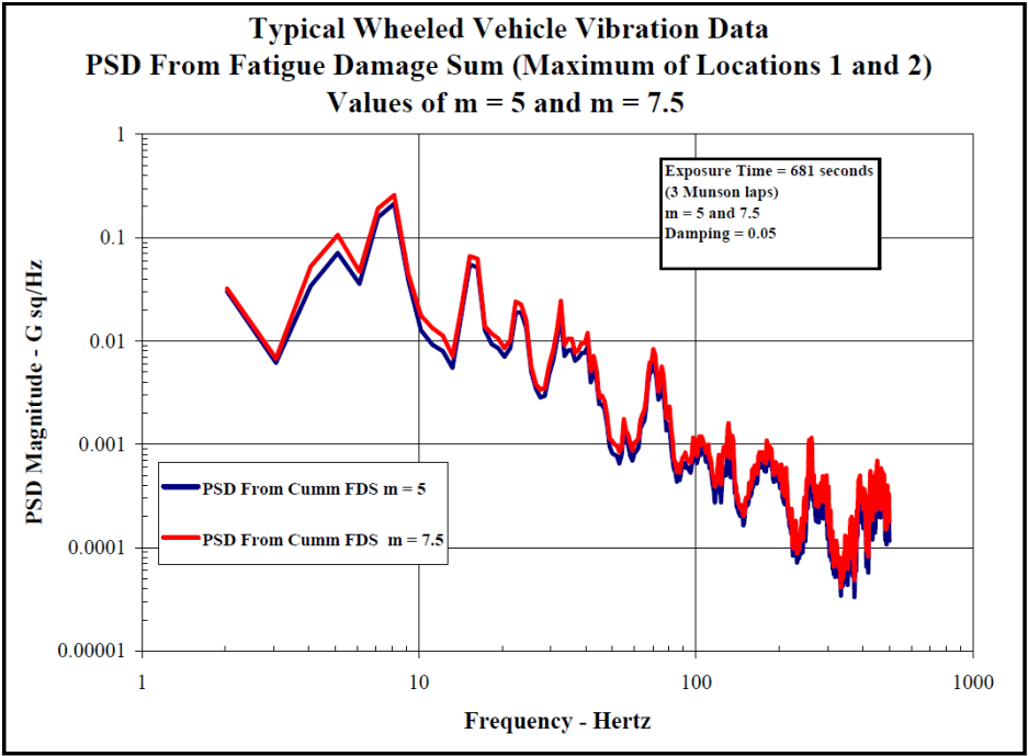
Figure description:
Typical Wheeled Vehicle Vibration Data", "subtitle": "PSD From Fatigue Damage Sum (Maximum of Locations 1 and 2\nValues of m = 5 and m = 7.5", "additional_notes": "The axes are on a logarithmic scale. Data values are estimated from the graph grid lines and represent key peaks and troughs to capture the profile of the fatigue damage sum spectrum. Red (m=7.5 shows higher sensitivity to peak values compared to blue (m=5.
PSD From Fatigue Damage Sum (Maximum of Locations 1 and 2
Legend
- PSD From Cumm FDS m = 5 — color: blue; symbol: Solid line
- PSD From Cumm FDS m = 7.5 — color: red; symbol: Solid line
Annotations
- Exposure Time = 681 seconds, (3 Munson laps, m = 5 and 7.5, Damping = 0.05 (text_label - position: top right box))
| Frequency - Hertz | PSD From Cumm FDS m = 5 | PSD From Cumm FDS m = 7.5 |
|---|---|---|
| 2.0 | 0.030 | 0.033 |
| 3.1 | 0.006 | 0.007 |
| 4.8 | 0.070 | 0.100 |
| 7.8 | 0.200 | 0.250 |
| 10.0 | 0.013 | 0.018 |
| 12.0 | 0.005 | 0.007 |
| 15.0 | 0.055 | 0.065 |
| 19.0 | 0.007 | 0.010 |
| 22.0 | 0.019 | 0.024 |
| 28.0 | 0.003 | 0.004 |
| 30.0 | 0.008 | 0.024 |
| 40.0 | 0.008 | 0.012 |
| 50.0 | 0.0008 | 0.0012 |
| 60.0 | 0.0008 | 0.0015 |
| 70.0 | 0.0055 | 0.0080 |
| 100.0 | 0.0005 | 0.0008 |
| 150.0 | 0.0008 | 0.0015 |
| 180.0 | 0.0006 | 0.0010 |
| 250.0 | 0.0007 | 0.0011 |
| 300.0 | 0.0002 | 0.0004 |
| 400.0 | 0.0002 | 0.0005 |
| 500.0 | 0.00015 | 0.0003 |
Figure 514.8F-C.7. Comparison of combined vibration power spectra developed from two exponents.
For this set of measured environments (acceleration spectra) and associated exposure times, the final combined spectrum is somewhat independent of the value of the exponent chosen. Forty percent of the spectral amplitudes for the two exponents were within 1 dB (based on m=7.5 as the reference), 80 percent were within 2 dB and all were within 2.4 dB.
Documentation of the spectral combination process, including assumptions (e.g., value of b), is essential. The final combined spectrum should be compared to the original input spectra to ensure that the resultant spectrum is a reasonable representation of the measured environment.
- FDS APPROACH TO DEVELOPMENT OF A LVTS.
In summarizing the example provided in the previous section, a single ASD was computed, representative of the ensemble of data acquired from making three passes over four specific road courses. The ASD derived from the inverse of the cumulative FDS is compared to the envelope of the data ensemble as shown in Figure 514.8F-C.5. From Figure 514.8F-C.7 it is clear that the spectral shapes and amplitudes are very similar for the ASD’s derived in the examples in previous section for both selections of m (m=5 and m=7.5). From Figure 514.8F-C.5 it is also clear that the ASD computed from the inverse cumulative FDS falls significantly below the envelope of the data ensemble. Employing equation 9.5, one could easily compress the test time by increasing the magnitude of the ASD. This can be accomplished by changing the T parameter of equation C.3. As in Annex F, paragraph 9, one should always use caution in employing time compression techniques. When dealing with data of a similar spectral characteristic, a conservative approach would be to limit the final compressed spectral shape to the spectral shape of the envelope of the original data ensemble. Reviewing the spectral shapes of the ASD’s computed from the inverse cumulative FDS and the envelope of the original data ensemble, it is clear that the ratio between the two curves is not the same at each spectral line. Therefore, one will need to set some criteria, which is often test specific, for addressing the amount of
MIL-STD-810H METHOD 514.8, ANNEX F, APPENDIX C
time compression employed. In the example discussed in this Appendix, the average ratio between 2 and 100 Hz was set at the compression ratio. This spectral band was considered to be of primary importance for this example since the data set was from a wheeled vehicle and the spectrum is dominated by energy below 100 Hz. Figure 514.8F-C.8 illustrates the effect of time compression based on the ratio described above. Using the time compressed spectral shape, the test time reduces from 681 seconds (the actual time spent on the courses) to either 72 seconds (when ) or 54 seconds (when ). As a final step, the analyst will usually reduce the number of breakpoints (smooth the spectral shape) while maintaining the overall G-rms level.
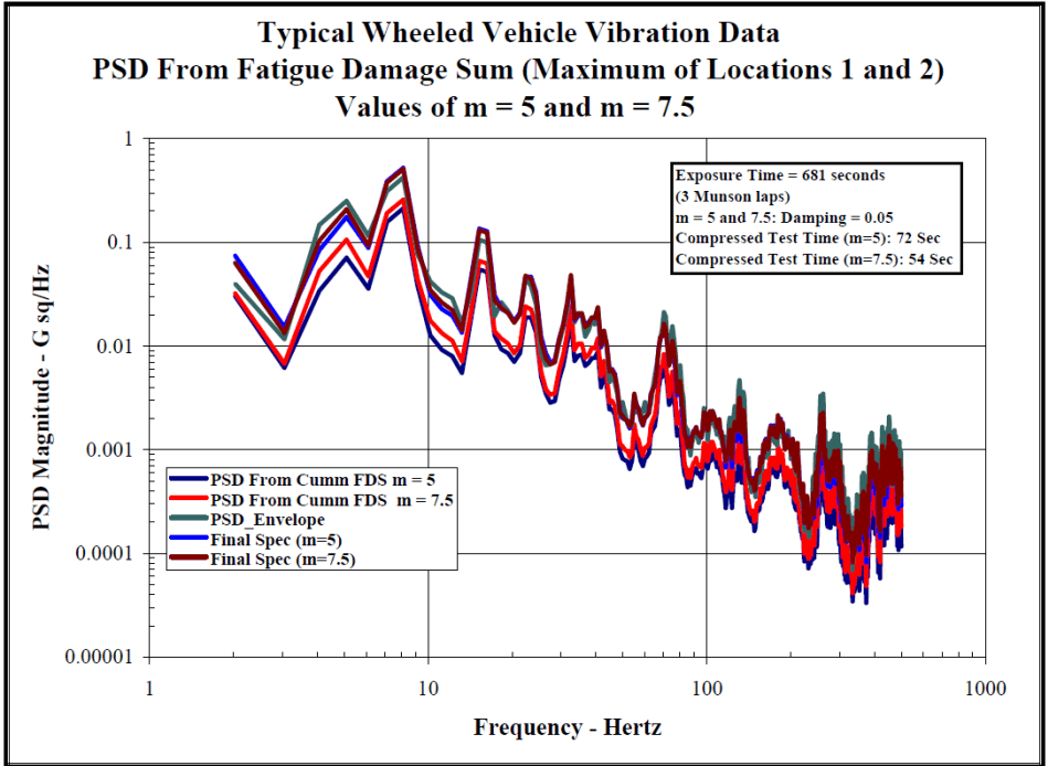
Figure description:
Typical Wheeled Vehicle Vibration Data Values of m = 5 and m = 7.5
PSD From Fatigue Damage Sum (Maximum of Locations 1 and 2
Legend
- PSD From Cumm FDS m = 5 — color: dark blue; symbol: solid line
- PSD From Cumm FDS m = 7.5 — color: red; symbol: solid line
- PSD_Envelope — color: teal; symbol: solid line
- Final Spec (m=5 — color: blue; symbol: solid line
- Final Spec (m=7.5 — color: dark red; symbol: solid line
Annotations
- Exposure Time = 681 seconds (3 Munson laps (text_label - position: top right box))
- m = 5 and 7.5; Damping = 0.05 (text_label - position: top right box)
- Compressed Test Time (m=5: 72 Sec (text_label - position: top right box))
- Compressed Test Time (m=7.5: 54 Sec (text_label - position: top right box))
| Frequency - Hertz | PSD From Cumm FDS m = 5 | PSD From Cumm FDS m = 7.5 | PSD_Envelope | Final Spec (m=5) | Final Spec (m=7.5) |
|---|---|---|---|---|---|
| 2.0 | 0.035 | 0.04 | 0.04 | 0.075 | 0.065 |
| 3.0 | 0.006 | 0.008 | 0.012 | 0.015 | 0.012 |
| 5.0 | 0.04 | 0.07 | 0.15 | 0.1 | 0.08 |
| 7.0 | 0.07 | 0.1 | 0.25 | 0.2 | 0.15 |
| 8.0 | 0.08 | 0.2 | 0.5 | 0.25 | 0.4 |
| 10.0 | 0.012 | 0.018 | 0.045 | 0.035 | 0.03 |
| 13.0 | 0.005 | 0.008 | 0.025 | 0.02 | 0.015 |
| 15.0 | 0.06 | 0.1 | 0.14 | 0.12 | 0.11 |
| 18.0 | 0.01 | 0.015 | 0.025 | 0.02 | 0.018 |
| 23.0 | 0.025 | 0.035 | 0.05 | 0.045 | 0.04 |
| 30.0 | 0.003 | 0.004 | 0.008 | 0.006 | 0.005 |
| 32.0 | 0.015 | 0.02 | 0.05 | 0.04 | 0.035 |
| 40.0 | 0.007 | 0.01 | 0.025 | 0.018 | 0.015 |
| 50.0 | 0.0008 | 0.0012 | 0.0035 | 0.0025 | 0.002 |
| 60.0 | 0.0007 | 0.001 | 0.003 | 0.002 | 0.0015 |
| 70.0 | 0.005 | 0.008 | 0.02 | 0.015 | 0.012 |
| 80.0 | 0.0006 | 0.0009 | 0.002 | 0.0015 | 0.0012 |
| 100.0 | 0.0004 | 0.0006 | 0.0025 | 0.002 | 0.0015 |
| 130.0 | 0.001 | 0.0015 | 0.005 | 0.0035 | 0.0025 |
| 200.0 | 0.0001 | 0.0002 | 0.002 | 0.0015 | 0.001 |
| 250.0 | 0.0005 | 0.0008 | 0.0035 | 0.0025 | 0.002 |
| 300.0 | 0.00004 | 0.00006 | 0.0015 | 0.001 | 0.0008 |
| 400.0 | 0.00006 | 0.0001 | 0.0018 | 0.0012 | 0.001 |
| 500.0 | 0.00015 | 0.00025 | 0.002 | 0.0015 | 0.0012 |
Notes: The y-axis is in a logarithmic scale for Power Spectral Density (G sq/Hz, and the x-axis is in a logarithmic scale for Frequency (Hz. Values in the table are approximate based on the plot.))
Figure 514.8F-C.8. Time compression of ASD's computed from the inverse cumulative fatigue damage spectrum.
This example is relatively simple; however, the techniques could easily be expanded to address more complex ensembles of data to include spectra with either narrowband or tonal components.
MIL-STD-810H METHOD 514.8, ANNEX F, APPENDIX D
Vibration Specification Development Procedure
514.8F -D.I. VSD Required Parameters
| Block Size | The number of data samples to include in ASD calculation. The block size is typically set equal to the sample rate to give a 1 second block and 1 Hz ASD resolution. |
|---|---|
| Window Type | The window type to use for ASD calculation, typically Hann. |
| Minimum g-rms threshold | Used to assure low level events will not overly affect LVTS ASD shape. The threshold |
| is set as a g-rms ratio (default 50%) of the maximum ASD in the group. | |
| Crest Factor Threshold | These thresholds can be used to alert the analyst if a section of data is grossly non-Gaussian. The analyst can then decide if the data should be excluded from the development process. |
| Skewness Threshold | |
| Kurtosis Threshold | |
| Start Frequency | This is the start frequency for the broadband portion of the LVTS. This is typically set to 5 Hz or the frequency of the lowest tonal component. |
| End Frequency | This is the upper limit of the LVTS bandwidth. This should be set by a review of the data. Typically used values include 200 Hz, 500 Hz, or 2000 Hz. |
| Nₑ, Nₛ | Analyst defined factors defining the number of standard deviations to use in the process (default = 1). Nₑ is for an individual event and Nₛ is for combining multiple events. |
| Mₑ, Mₛ | Analyst defined factors to limit conservatism in the process. Mₑ is for an individual event and Mₛ is for combining multiple events. |
| DC Component | Remove the DC components from the time domain data before calculation of ASDs. The DC component is often a result of signal conditioner offset and can be removed without affecting LVTS development. |
514.8F -D.II. Single-Event ASD Sum-Set
| Nomenclature | Definition |
|---|---|
| ASD(Avg) | A standard nd average ASD. (See Gm (f) as defined in Appendix B) |
| ASD(Peak) | Calculated by holding the maximum amplitude of each spectral line over nd averages. (See Gp (f) as defined in Appendix B) |
| ASD(Stdv) | Calculated by determining the standard deviation of each spectral line over n averages. (See Gd (f) as defined in Appendix B) |
| ASD(Sum) | Calculated by adding Ne standard deviations to the average for each spectral line. ASD(Sum) = Ne *ASD(Stdv) + ASD(Avg) Ne is a user defined variable typically set to 1. ASD(Sum) is limited by ASD(Peak) and Me *ASD(Avg) where Me is a user defined variable typically set to 2. (See Gs (f) as defined in Appendix B) |
| ASD(SpkRmvd) | ASD(Sum) after Frequency Spectral spike Removal. |
514.8F -D.III. Spectral Spike Removed Table, Average
| Project File: | Example Wheeled Vehicle | [ ] | |||||
|---|---|---|---|---|---|---|---|
| Total Miles: | 1000 | Block size : | 4096 | Start Freq: 3 | Raw ASD | W-UCol ASD | |
| Date Proc :9/16/2002 | Window Type: | Hann | End Frq: 500 | N: | 1 | 1 | |
| Time Proc :6:37:44 AM | Min g-rms: | 0.5 | Rmv DC : Y | M: | 2 | 2 | |
| Total G-RMS of removed Spectral spike | |||||||
| Channel | 1 | 2 | 3 | ||||
| Description | Channel 1 | Channel 2 | Channel 3 | ||||
| Type | ASD(Avg) | ASD(Avg)| | ASD(Avg) | ||||
| Test Time | 30 | 30 | 30 | ||||
| Event | Beta Dist Time | Center Freq | Bandwidth Selected | g-rms | g-rms | g-rms | |
| 1 Harmonic | 5 mph 2" WB | 8.31 | 3.67 | 6 | 0.1534 | 2.79E-02 | 5.31E-02 |
| 7.5 mph 2" WB | 21.28 | 5.50 | 5 | 0.2691 | 3.41E-02 | 0.134565 | |
| 10 mph 2" WB | 7.47 | 7.33 | 7 | 0.5755 | 8.74E-02 | 0.5730498 | |
| 2 Harmonic | 5 mph 2" WB | 8.31 | 7.33 | 6 | 0.1118 | 3.49E-02 | 7.37E-02 |
| 7.5 mph 2" WB | 21.28 | 11.00 | 7 | 8.72E-02 | 3.22E-02 | 5.18E-02 | |
| 10 mph 2" WB | 7.47 | 14.67 | 6 | 8.98E-02 | 2.67E-02 | 0.211421 | |
| 3 Harmonic | 5 mph 2" WB | 8.31 | 11.00 | 6 | 0.06546 | 4.01E-02 | 9.12E-02 |
| 7.5 mph 2" WB | 21.28 | 16.50 | 9 | 2.63E-02 | 2.94E-02 | 0.05846 | |
| 10 mph 2" WB | 7.47 | 22.00 | 8 | 3.08E-02 | 3.75E-02 | 0.07558 | |
514.8F -D.V. Runtime Calculation
| Event No | Event Name | Scenario Time | 1 (Min) | 2 (Min) | 3 (Min) | 4 (Min) | 5 (Min) | 6 (Min) | 7 (Min) |
|---|---|---|---|---|---|---|---|---|---|
| 1 | Radial Washboard 5 MPH | 6.62 | 0.0000 | 0.0000 | 0.0000 | 0.0000 | 0.0000 | 0.0000 | 0.000 |
| 2 | Radial Washboard 10 MPH | 9.76 | 1.0839 | 0.0000 | 7.5042 | 1.4266 | 0.0000 | 5.0242 | 0.000 |
| 3 | Radial Washboard 15 MPH | 3.51 | 44.0730 | 16.5723 | 67.7850 | 42.9182 | 31.0571 | 17.1557 | 33.406 |
| 4 | Embedded Rock 5 MPH | 9.01 | 0.0000 | 0.0000 | 0.0000 | 0.0000 | 0.0000 | 0.0000 | 0.648 |
| 5 | Embedded Rock 7.5 MPH | 11.04 | 6.5395 | 4.8474 | 4.7421 | 6.0680 | 3.1819 | 0.0000 | 21.373 |
| 6 | Embedded Rock 10 MPH | 4.74 | 46.1231 | 31.9828 | 10.4189 | 34.8946 | 6.6298 | 0.0000 | 38.806 |
| 7 | Belgian Block 5 MPH | 1.05 | 0.0000 | 0.0000 | 0.0000 | 0.0000 | 0.0000 | 0.0000 | 0.000 |
| 8 | Belgian Block 10 MPH | 3.24 | 0.0000 | 0.0000 | 0.0000 | 0.0000 | 0.0000 | 0.0000 | 0.000 |
| 9 | Belgian Block 15 MPH | 5.18 | 0.0000 | 0.0000 | 0.0000 | 0.0000 | 0.0000 | 0.0000 | 0.846 |
| 10 | Belgian Block 20 MPH | 5.02 | 2.2310 | 0.5887 | 0.9003 | 2.5947 | 3.1033 | 0.0000 | 2.898 |
| 11 | Belgian Block 25 MPH | 1.88 | 17.4201 | 4.2217 | 6.0418 | 16.9478 | 14.9296 | 0.0000 | 6.81 |
| TF | 117.4706 | 58.2131 | 97.3924 | 104.8499 | 58.9017 | 22.1799 | 104.791 | ||
| TFA | 60 | 30 | 60 | 30 | 30 | 15 |
MIL-STD-810H METHOD 514.8, ANNEX F, APPENDIX D
514.8F -D.VI. Group Sum-Set Definition
| ASD(Avg_g) | The weighted average of the ASD group. See Equation D.2-1. (See Ga(f) as defined in Appendix B) |
| ASD(Peak_g) | Calculated by holding the maximum amplitude of each spectral line over all events. |
| ASD(Stdv_g) | The weighted standard deviation of the ASD group. See Equation D2.2-3. (See Ge(f) as defined in Appendix B) |
| ASD(Sum_g) | Calculated by adding Ng standard deviations to the average for each spectral line. ASD(Sum_g) = Ng *ASD(Stdv_g) + ASD(Avg_g) Calculated by adding Ng standard deviations to the average for each spectral line. ASD(Sum) = Ng *ASD(Stdv) + ASD(Avg) Ng is a user defined variable typically set to 1. ASD(Sum) is limited by ASD(Peak) and Mg *ASD(Avg) where Mg is a user defined variable typically set to 2. (See Gf(f) as defined in Appendix B "for N=1") |
| ASD(Final) | The ASD(Sum_g) scaled to a user selected final time. |
The ASDs of the group sum-set, as with the single-event ASD sum-set, are calculated on a spectral line basis. The ASD(Avg_g) is an average of the ASD(SpkRmvd) for all events in the group (excluding those for which the g-rms is below the user defined threshold). Unlike the ASD(Avg) of the single-event ASD sum-set, the ASD(Avg_g) is not a standard n average ASD. Instead, the individual ASDs are weighted to the factors defined in the scenario table (see Table 514.8F-D.IV). Typically, the weighting factors are set equal to the individual event scenario times. The idea of a weighted approach is to produce a time-based calculation instead of an event-based calculation. In effect, weighting to the scenario time produces a separate ASD for each minute of the lifecycle, instead of an ASD for each event. Each minute of the system’s lifecycle would then be weighted equally in determining the average. A similar method is used to calculate the standard deviation of the group ASD(Stdv_g).
Assuming there are n events that exceed the minimum g-rms, that is weighting factor of each event, and that is the level of each event, then for each spectral line:
| ASD(Avg_g) = n ∑WiGi i=1 n ∑Wi i=1 | D.2-1 |
MIL-STD-810H METHOD 514.8, ANNEX F, APPENDIX D
D.2-2
The ASD(Sum_g) is calculated by adding N g standard deviations to the average, where N g is a user defined variable typically set to 1. Use of the ASD(Sum_g) is intended to account for factors such as differences in road surfaces, driver variances, and consideration of road surfaces not included in the data acquisition phase and other relevant variables. The ASD(Sum_g) is constrained to be no higher than M g *ASD(Avg_g) where M g is a user defined parameter with a default value of 2.0. The ASD(Sum_g) is also limited to the ASD(Peak_g) level at each spectral line. Although some additional processing may be required, the ASD(Sum_g) coupled with the runtime calculated in the previous step now represent the equivalent lifetime fatigue of an item mounted at that location. Recall that each channel represents a vibration axis for a given location. The ASD(Sum_g) becomes the working ASD and is passed forward to the next step.
In some cases multiple channels (or locations) must be combined into a single LVTS. This can be accomplished by simply enveloping the channels later in the VSD process. However, it is possible to combine multiple channels concurrently with the event combination. Assuming j is a list of m channels to combine, then for each spectral line:
D.2-3 D.2-4
514.8F -D.IX. LVTS Combination Example
| Freq | LVTS01 | LVTS02 | Norm Level | LVTS01 New Time | LVTS02 New Time | Total New Time | Final Run Time | LVTS_C |
|---|---|---|---|---|---|---|---|---|
| (Hz) | (G²/Hz) | (G²/Hz) | (G²/Hz) | (min) | (min) | (min) | (min) | (G²/Hz) |
| 5 | 0.100 | 0.200 | 0.200 | 2.23 | 15.00 | 17.23 | 20.00 | 0.208 |
| 6 | 0.200 | 0.400 | 0.400 | 2.23 | 15.00 | 17.23 | 20.00 | 0.415 |
| 7 | 0.300 | 0.400 | 0.400 | 10.20 | 15.00 | 25.20 | 20.00 | 0.459 |
| 8 | 0.400 | 0.400 | 0.400 | 30.00 | 15.00 | 45.00 | 20.00 | 0.536 |
| 9 | 0.400 | 0.300 | 0.300 | 88.24 | 15.00 | 103.23 | 20.00 | 0.501 |
This method can also be used this to combine multiple events into a broadband LVTS, replacing the steps outline in paragraphs 2.6 through 2.8 above. An alternate method to add conservatism must be found, and care should be taken to assure the method does not corrupt the overall shape of the ASD set. Refer to paragraph 2.2.1 (main body of Method 514) for cautions associated with combining LVTS.
Downloaded from https://www.everyspec.com
MIL-STD-810H
METHOD 514.8, ANNEX F, APPENDIX D
(This page is intentionally blank.)