The documents listed in this section are specified in sections 3, 4, or 5 of this Standard. This section does not include documents cited in other sections of this Standard or recommended for additional information or as examples. While every effort has been made to ensure the completeness of this list, document users are cautioned that they must meet all specified requirements of documents cited in sections 3, 4, or 5 of this Standard, whether or not they are listed.
2.1.1
Effects of the Contaminating Fluids Environment
During its life cycle, materiel may be accidentally or intentionally exposed to one or more fluids that could have an adverse effect on the materiel. As a result, exposure of materiel to contaminating fluids may either temporarily or permanently impair the operation of the materiel by changing the physical properties of the material(s) composing it. Consider the following typical examples of problems to help determine if this Method is appropriate for the materiel being tested. The list is not intended to be all-inclusive and some of the examples may overlap.
a. Physical
- (1) Shattering of glass vials and optical materiel.
- (2) Binding or slackening of moving parts.
- (3) Cracking of solid pellets or grains in explosives.
- (4) Differential contraction or expansion rates or induced strain rates of dissimilar materials.
MIL-STD-810H
METHOD 504.3
- (5) Deformation or fracture of components. (Solder reflow is the worst case.)
- (6) Cracking of surface coatings.
- (7) Seal or gasket failures (leaking of sealed compartments).
- (8) Failure of insulation protection.
- (9) Condensation of water onto cold surfaces suddenly exposed to higher ambient temperatures at "high relative humidity" - can cause frosting on optical surfaces - can cause corrosion on vulnerable surfaces.
- (10) Differential contraction or expansion rates or induced strain rates between surface and interior portions of thermally massive constructs.
- (11) Packaging failure.
- (12) Crazing or swelling of plastics and rubbers.
- (13) Adhesion failures (delamination).
- (14) Paint/legend removal.
- b. Chemical.
- (1) Separation of constituents.
- (2) Failure of chemical agent protection.
- (3) Leeching of antioxidants and other soluble materials.
- (4) Corrosion.
- (5) Melting or decomposition.
- c. Electrical.
- (1) Changes in electrical and electronic components.
- (2) Electronic or mechanical failures due to rapid water or frost formation.
- (3) Excessive static electricity.
- (4) Interruption of electrical continuity (such as "grounding" fingers on EMI strips).
- (5) Increase in electrical resistance due to thermo-mechanical "fretting corrosion."
2.1.2
Mission/field transportation. This involves movement of materiel as cargo where the platform may be two-wheeled trailers, 2-1/2 to 10 ton trucks, and/or semi-trailers. Typical distances for this phase are 480 to 800 kilometers (300 to 500 miles). Road conditions for mission/field support differ from the common carrier in that, in addition to the paved highway, the vehicles will traverse unimproved roads and unprepared terrain (off-the-road) under combat conditions.
2.1.3
Exposure levels. Whenever possible, measure vibration on the transport vehicles using the road conditions (surfaces, speeds, and maneuvers) of the materiel’s LCEP. Include realistic load configurations (approximately 75 percent of the vehicle load capacity by weight). Use these data to develop exposure levels per Annex F. Alternatively, derive exposure levels as discussed below.
|
a. Truck transportation over US highways. Derive exposure levels from Figure 514.8C-2 and Table 514.8C-I, or, if the test item orientation is unknown or variable see Figure 514.8C-3 and Table 514.8C-II for exposure levels. These figures are based on data measured at the cargo floor of seven different configurations of trucks and semitrailer combinations. Both conventional suspensions and air-cushioned suspensions are represented. The data were collected from typical interstate highways (including rough portions as part of the database).
Test Schedule: Secured Cargo – Common Carrier (See paragraph 6.1, reference oo.)
Vehicles Used for Composite: This schedule is based on data measured at the cargo floor of seven different configurations of trucks and semitrailer combinations. Both conventional suspensions and air-cushioned suspensions are represented. The data were collected from typical interstate highways with rough portions as part of the database:
Measured Locations: Measurements were made on the cargo floor of the vehicles tested.
Type of Test Load: Unknown.
Scenario to be Simulated: 1609 km (1000 miles) on interstate highways.
Assumptions (Scenario, Load, Failure Mechanism, etc.):
100 percent of scenario is on improved interstate highways
Fatigue is the failure mode
Test Time Compression: This test represents 1609 km (1000 mi) in 60 minutes so there is time compression involved. The algorithm used to determine the exaggeration factor is unknown.
Test Time: 60 minutes per axis
Exaggeration Factor: Unknown
Method of Combination of Spectra: Unknown.
Location of Control Accelerometer(s): 2 accelerometers at opposite corners, within 30 cm (12 in.) from test item
Recommended Control Scheme: Average (Extremal control may be appropriate for some applications)
For movement direction definitions, see paragraph 4.4 in the front part of this Method.
RMS Acceleration:1,2 (G-rms): Vertical – 1.08;
Transverse – 0.21; Longitudinal – 0.76; Envelope – 1.17.
Velocity (in/sec) (peak single amplitude): 1,2
Vertical – 9.68; Transverse – 1.23; Longitudinal – 6.11; Envelope – 9.69.
MIL-STD-810H METHOD 514.8, ANNEX C Displacement (in) (peak double amplitude): 1,2
Vertical – 0.37
Transverse - 0.04;
Longitudinal - 0.24;
Envelope – 0.37.
^1 Approximate values for a Gaussian random distribution which may vary based on the control system and spectral resolution. Peak velocity and displacement values are based on an acceleration maximum of three times the standard deviation (3σ) and a spectral resolution of 1 Hz.
2 For test items for which the test item orientation is unknown or variable the Envelope profile should be run for all three axes (Figure 514.8C-3 and Table 514.8C-II).
MIL-STD-810H METHOD 514.8, ANNEX C
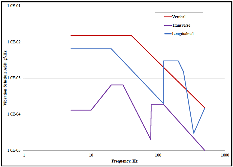
Figure description:
Vibration Schedule ASD vs. Frequency
Vibration Schedule ASD vs. Frequency
Legend
- Vertical — color: red; symbol: solid line with square markers
- Transverse — color: purple; symbol: solid line with triangle markers
- Longitudinal — color: blue; symbol: solid line with diamond markers
| Frequency (Hz) | Vertical (g²/Hz) | Transverse (g²/Hz) | Longitudinal (g²/Hz) |\n| :--- | :--- | :--- | :--- |\n| 5 | 1.50E-02 | 1.25E-04 | 6.50E-03 |\n| 10 | 1.50E-02 | 1.25E-04 | 6.50E-03 |\n| 20 | 1.50E-02 | 6.50E-04 | 6.50E-03 |\n| 30 | 1.50E-02 | 6.50E-04 | 3.00E-03 |\n| 40 | 1.50E-02 | 2.30E-04 | 1.70E-03 |\n| 78 | 4.40E-03 | 2.00E-05 | 4.70E-04 |\n| 78 | 4.40E-03 | 1.90E-04 | 4.70E-04 |\n| 120 | 2.00E-03 | 1.90E-04 | 2.00E-04 |\n| 120 | 2.00E-03 | 1.90E-04 | 3.00E-03 |\n| 200 | 7.80E-04 | 6.50E-05 | 3.00E-03 |\n| 240 | 5.60E-04 | 4.50E-05 | 1.60E-03 |\n| 350 | 2.80E-04 | 2.00E-05 | 3.00E-05 |\n| 500 | 1.50E-04 | 1.00E-05 | 1.50E-04 |
Notes: The chart utilizes a log-log scale for both axes. Values in the table are estimated based on visual inspection of major and minor grid lines. Vertical jumps in the Transverse and Longitudinal data series at 78 Hz and 120 Hz respectively are represented by duplicated frequency rows.
Figure 514.8C-2 – Category 4 – Common carrier (US highway truck vibration exposure).
| Vertical | Transverse | Longitudinal | |||
|---|---|---|---|---|---|
| Frequency, Hz | ASD, g²/Hz | Frequency, Hz | ASD, g²/Hz | Frequency, Hz | ASD, g²/Hz |
| 5 | 0.015 | 5 | 0.00013 | 5 | 0.0065 |
| 40 | 0.015 | 10 | 0.00013 | 20 | 0.0065 |
| 500 | 0.00015 | 20 | 0.00065 | 120 | 0.0002 |
| 30 | 0.00065 | 121 | 0.003 | ||
| 78 | 0.00002 | 200 | 0.003 | ||
| 79 | 0.00019 | 240 | 0.0015 | ||
| 120 | 0.00019 | 340 | 0.00003 | ||
| 500 | 0.00001 | 500 | 0.00015 | ||
| rms = 1.08 g | rms = 0.21 g | rms = 0.76 g | |||
MIL-STD-810H METHOD 514.8, ANNEX C
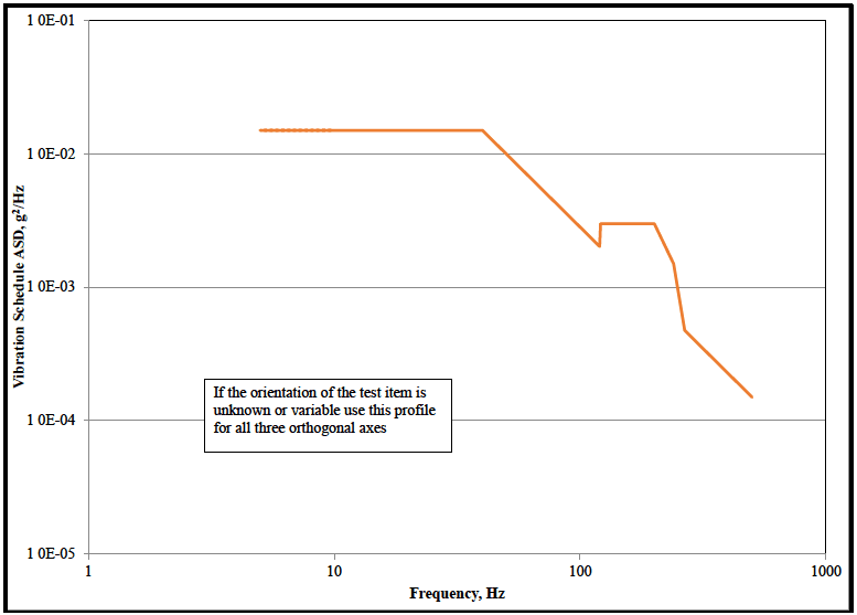
Figure description:
Annotations
- If the orientation of the test item is unknown or variable use this profile for all three orthogonal axes (text_label - position: Centered in a text box at approximately x=25, y=3E-04)
| Frequency (Hz) | Vibration Schedule ASD (g²/Hz) |
|---|---|
| 5 | 1.5E-02 |
| 40 | 1.5E-02 |
| 120 | 2.0E-03 |
| 120 | 3.0E-03 |
| 200 | 3.0E-03 |
| 240 | 1.5E-03 |
| 280 | 5.0E-04 |
| 500 | 1.5E-04 |
Notes: The chart is a log-log plot representing a vibration test profile (ASD vs. Frequency.)
Figure 514.8C-3 - Category 4 - Common carrier for unknown orientation (US highway truck vibration exposure).
| Envelope | |
|---|---|
| Frequency, Hz | ASD, g2/Hz |
| 5 | 0.015 |
| 40 | 0.015 |
| 120 | 0.002025 |
| 121 | 0.003 |
| 200 | 0.003 |
| 240 | 0.0015 |
| 266 | 0.000475 |
| 500 | 0.00015 |
| rms = 1.17 g | |
b. Two-wheeled trailer and wheeled vehicles
Both trucks and two-wheeled trailers are used between the Forward Supply Point (FSP) and at the Using Unit (USU). When materiel is too large for the two-wheeled trailer, use the composite wheeled levels.
(1) Two wheeled trailer (TWT). Exposures are shown in Figure 514.8C-4, and are followed by the respective data table (Table 514.8C-IV). If the orientation of the test item is unknown or variable see Figure 514.8C-5 and Table 514.8C-V for exposure levels. (See paragraph 6.1, references pp to vv.)
Test Schedule: Secured Cargo – Two-Wheeled Trailer
Vehicles Used for Composite: Measured vibration data from the following vehicles (Table 514.8C-III) were used to develop the Two-Wheeled Trailer Vehicle test schedule:
| NOMENCLATURE | DESCRIPTION |
|---|---|
| M105A2 | U.S. 1-1/2 ton trailer |
| N/A | German 1-1/2 ton trailer |
| M1102 | U.S. 1-1/4 ton trailer |
Measured Locations: 9 locations on frame under cargo bed (3X3 matrix).
Type of Test Load: Sand filled ammo boxes (or other similar cargo) were secured to the cargo bed, and loaded to 34 of vehicle rated load.
Scenario to be Simulated: 51.5 km (32 mi) from the forward supply point to the using unit described as follows: The typical mission/field transport scenario starts at the port staging area (PSA). The movement prior to this point would include transport by commercial common carrier, military long-range aircraft, ship, and/or railroad. This movement would occur over improved road surfaces or in platforms that have been proven to impose significantly lower vibration levels than those vehicles used for transport from the port staging area to the using unit. The typical scenario has established that 51.5 km (32 mi) of transport are expected between forward supply point to the using unit. This transport is in two-wheeled trailers. The road surfaces will be paved, secondary, and cross-country.
Assumptions (Scenario, Load, Failure Mechanism, etc.):
Total Mission of 51.5 km (32 miles) is accounted for as follows:
- • 15 percent of total mission, 7.7 km (5 miles), is on-road and considered benign compared to the off-road environment.
- • 85 percent of total mission, 43.8 km (27 miles), is off-road:
- One-third of the off-road environment, 14.6 km (9 miles), is rough terrain consistent with the Belgian Block, Two-Inch Washboard, Radial Washboard, and Three-Inch Space Bump courses used to collect data. Average Speed over these courses was 26 km/hr (16 mph).
- Two-thirds of the off-road environment, 29.2 km (18 miles), is considered benign compared to the test conditions described above.
Failure mode: fatigue
Test Time Compression: None; this test is run in real time.
Test Time: 32 minutes per axis
Exaggeration Factor: 1.00
MIL-STD-810H
METHOD 514.8, ANNEX C
Method of Combination of Spectra: A statistical method as described in Annex F, Appendix C,
- was used to create the spectra for the individual trailers in Table 514.8C-III. This method makes use of the spectral variance from different measurement locations and test conditions and produces a spectrum that is a very conservative estimate of the actual measured environments. This procedure produced an ASD for each trailer in each of the orthogonal axes. The composite two-wheeled trailer spectrum was created by enveloping the individual trailers. Ideally a statistical method would have been used (as was done for the Composite Wheeled Vehicle below) but because the number of samples was so low an enveloping method was employed.
- Location of Control Accelerometer(s): 2 accelerometers at opposite corners, within 30 cm (12 in.) from test item
Recommended Control Scheme: Average (Extremal control may be appropriate for some
- applications). Based on the field data characteristics and the conservatism associated with the composite vehicle VSD process, drive limiting to 3 sigma is recommended.
For movement direction definitions, see paragraph 4.4 in the front part of this Method.
| RMS Acceleration:1,3 (G-rms): | |
| Vertical | – 3.98; |
| Transverse | – 1.22; |
| Longitudinal | – 2.52; |
| Envelope | – 4.03. |
| Velocity (in/sec) (peak single amplitude):1,3 | |
| Vertical | – 33.29; |
| Transverse | – 15.23; |
| Longitudinal | – 18.18; |
| Envelope | – 33.30. |
| Displacement (in) (peak double amplitude):1,2,3 | |
| Vertical | – 1.51; |
| Transverse | – 0.69; |
| Longitudinal | – 0.79; |
| Envelope | – 1.51. |
^1 Approximate values for a Gaussian random distribution which may vary based on the control system and spectral resolution. Peak velocity and displacement values are based on an acceleration maximum of three times the standard deviation (3σ) and a spectral resolution of 1 Hz.
² For shaker systems that are incapable of the displacement requirements of this schedule, minor adjustments may be made to the low frequency within the tolerances specified in 4.2.2.1a (main body) to accommodate the shaker limitations. If any schedule needs to be modified, make sure that all parties involved (tester, customer, etc.) are aware of the reason for the changes, and agree to the changes prior to test. Ensure an adequate test is performed and all deviations from the published schedules are properly documented.
³ For test items for which the test item orientation is unknown or variable the Envelope profile should be run for all three axes (Figure 514.8C-5 and Table 514.8C-V).
|
MIL-STD-810H METHOD 514.8, ANNEX C
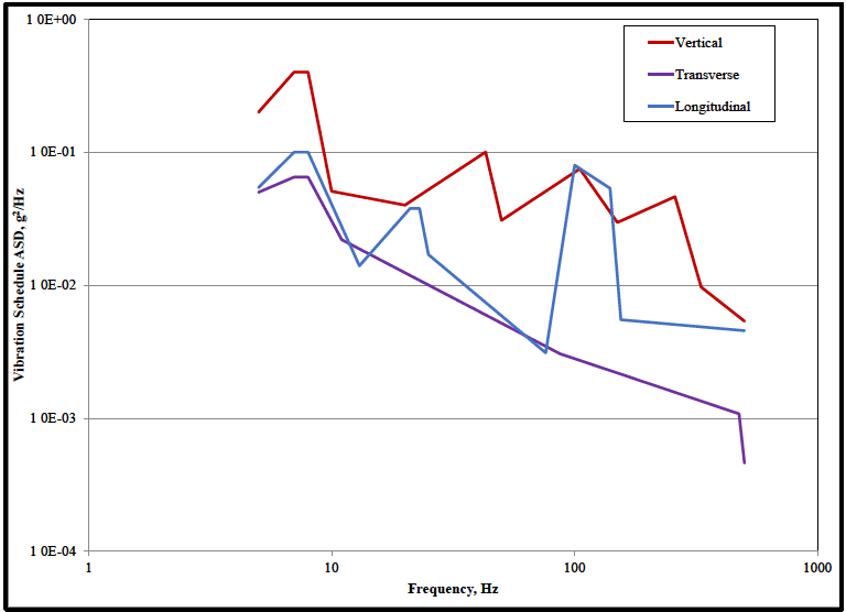
Figure description:
Vibration Schedule ASD
Vibration Schedule ASD vs. Frequency
Legend
- Vertical — color: red; symbol: Solid line
- Transverse — color: purple; symbol: Solid line
- Longitudinal — color: blue; symbol: Solid line
| Frequency (Hz) | Vertical (g²/Hz) | Transverse (g²/Hz) | Longitudinal (g²/Hz) |
|---|---|---|---|
| 5 | 0.2 | 0.052 | 0.056 |
| 7 | 0.4 | null | 0.1 |
| 8 | 0.4 | 0.066 | 0.1 |
| 8.5 | null | null | 0.1 |
| 10 | 0.052 | null | null |
| 11 | null | 0.024 | null |
| 13 | null | null | 0.014 |
| 20 | 0.04 | null | null |
| 22 | null | null | 0.038 |
| 25 | null | null | 0.038 |
| 27 | null | null | 0.017 |
| 45 | 0.1 | null | null |
| 50 | 0.031 | null | null |
| 75 | null | 0.0032 | 0.0032 |
| 100 | 0.075 | null | 0.08 |
| 140 | null | null | 0.055 |
| 150 | 0.03 | null | 0.0056 |
| 280 | 0.046 | null | null |
| 350 | 0.01 | null | null |
| 480 | null | 0.0011 | null |
| 500 | 0.0055 | 0.00046 | 0.0047 |
Notes: The axes for both Frequency and Vibration Schedule ASD are logarithmic. Data points are estimated based on visual interpretation of the log scales.
Figure 514.8C-4. - Category 4 - Composite two-wheeled trailer vibration exposure.
| Vertical | Transverse | Longitudinal | |||
|---|---|---|---|---|---|
| Frequency, Hz | ASD, g²/Hz | Frequency, Hz | ASD, g²/Hz | Frequency, Hz | ASD, g²/Hz |
| 5 | 0.20000 | 5 | 0.05000 | 5 | 0.05418 |
| 7 | 0.40000 | 7 | 0.06500 | 7 | 0.10000 |
| 8 | 0.40000 | 8 | 0.06500 | 8 | 0.10000 |
| 10 | 0.05090 | 11 | 0.02200 | 13 | 0.01400 |
| 20 | 0.04000 | 87 | 0.00306 | 21 | 0.03780 |
| 43 | 0.10036 | 475 | 0.00108 | 23 | 0.03780 |
| 50 | 0.03079 | 500 | 0.00046 | 25 | 0.01700 |
| 105 | 0.07500 | 76 | 0.00310 | ||
| 150 | 0.02964 | 100 | 0.08000 | ||
| 259 | 0.04636 | 140 | 0.05354 | ||
| 332 | 0.00970 | 155 | 0.00551 | ||
| 500 | 0.00537 | 500 | 0.00456 | ||
| rms = 3.98 g | rms = 1.22 g | rms = 2.52 g | |||
MIL-STD-810H METHOD 514.8, ANNEX C
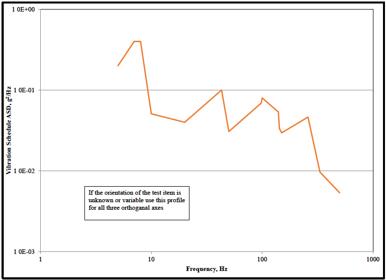
Figure description:
Vibration Schedule Profile Vibration profile for test item orientation
Vibration Schedule ASD vs. Frequency
Annotations
- If the orientation of the test item is unknown or variable use this profile for all three orthogonal axes (text_label - position: Centered at approximately x=25 Hz, y=0.005 g²/Hz)
| Frequency (Hz) | Vibration Schedule ASD (g²/Hz) |
|---|---|
| 5 | 0.2 |
| 7 | 0.4 |
| 8 | 0.4 |
| 10 | 0.05 |
| 20 | 0.04 |
| 43 | 0.1 |
| 48 | 0.03 |
| 100 | 0.08 |
| 140 | 0.055 |
| 145 | 0.03 |
| 260 | 0.045 |
| 320 | 0.01 |
| 500 | 0.005 |
Notes: The data is plotted on a log-log scale. Coordinates of vertices are estimated based on visual alignment with the log grid. Significant points on grid lines: (10, 0.05, (43, 0.1, (100, 0.08, (320, 0.01.))))
Figure 514.8C-5.- Category 4 – Composite two-wheeled trailer vibration exposure for unknown orientation.
| V, L&T Envelope | |
|---|---|
| Frequency, Hz | ASD, g²/Hz |
| 5 | 0.20000 |
| 7 | 0.40000 |
| 8 | 0.40000 |
| 10 | 0.05090 |
| 20 | 0.04000 |
| 43 | 0.10036 |
| 50 | 0.03079 |
| 98 | 0.06910 |
| 100 | 0.08000 |
| 140 | 0.05354 |
| 143 | 0.03350 |
| 150 | 0.02964 |
| 259 | 0.04636 |
| 332 | 0.00970 |
| 500 | 0.00537 |
| rms = 4.03 g | |
(2) Composite wheeled vehicle (CWV). Exposures are shown in Figure 514.8C-6, and are followed by the respective data table (Table 514.8C-VII). If the orientation of the test item is unknown or variable, see exposure levels shown in Figure 514.8C-7 and Table 514.8C-VIII. (See paragraph 6.1, references pp to vv.)
Test Schedule: Secured Cargo - Composite Wheeled Vehicle
Vehicles Used for Composite: Measured vibration data from the following vehicles (Table 514.8C-VI) were used to develop the Composite Wheeled Vehicle test schedule:
| NOMENCLATURE | DESCRIPTION |
|---|---|
| M985 | US Heavy Expanded Mobility Tactical Truck (HEMTT) 10-ton truck |
| MK27* | US Medium Tactical Vehicle Replacement (MTVR) 7-ton truck |
| M1083/M1084/M1085 | US Medium Tactical Vehicle (MTV) 5-ton truck |
| M1151**/M1152/M1113 | US High Mobility Multipurpose Wheeled Vehicle (HMMWV) 1-1/4-ton truck |
| M1074/M1075 | US Palletized Loading System (PLS) truck |
| M1078*** | US Light MTV 2-1/2-ton truck |
| MTVR-T* | US MTVR trailer |
| M989**** | US Heavy Expanded Mobility Trailer (HEMAT) |
| M1076 | US PLS trailer |
| M1095 | US MTV 5-ton trailer |
| M1082*** | US Light MTV 2-1/2-ton trailer |
| M871A3***** | US 22-ton semitrailer |
| Unimog | German 2-ton truck |
| Machine Fabrik Augsburg Nurnberg (MAN) | German 5-, 7-, 10-, 15-ton trucks |
| * | 2 measurement locations |
| ** | 6 measurement locations |
| *** | 8 measurement locations |
| **** | 4 measurement locations |
| ***** 12 measurement locations | |
Measured Locations: 9 locations on frame under cargo bed (3X3 matrix) except as noted in the table above
Type of Test Load: Sand filled ammo boxes (or other similar cargo) were secured to the cargo bed, and loaded to 3/4 of vehicle rated load.
Scenario to be Simulated: 805 km (500 mi) from the port staging area to the forward supply point described as follows: The typical mission/field transport scenario starts at the port staging area (PSA). The movement prior to this point would include transport by commercial common carrier, military long range aircraft, ship, and/or railroad. This movement would occur over improved road surfaces or in platforms that have been proven to impose significantly lower vibration levels than those vehicles used for transport from the port staging area to the using unit. The typical scenario has established that 805 km of transport are expected between the PSA and the forward supply point (FSP). This transport is in trucks and/or semitrailers. The road surfaces will be paved, secondary, and cross country.
MIL-STD-810H
METHOD 514.8, ANNEX C
Assumptions (Scenario, Load, Failure Mechanism, etc.):
Total Mission of 805 km (500 miles) is accounted for as follows:
- • 35 percent of total mission, 282 km (175 miles), is on-road and considered benign compared to the off-road environment.
- • 65 percent of total mission, 523 km (325 miles), is off-road:
- One-third of the off-road environment, 174 km (108 miles), is rough terrain consistent with the Belgian Block, Two-Inch Washboard, Radial Washboard, and Three-Inch Spaced Bump courses used to collect data. Average Speed over these courses was 26 km/hr (16 mph).
- Two-thirds of the off-road environment, 349 km (217 miles), is considered benign compared to the test conditions described above.
Failure mode: fatigue
Test Time Compression: Test time was computed from:
Where: = equivalent test time = in-service time for specified condition = ASD at test condition, = ASD at in-service condition, = 7.5 (see paragraph 2.2 of Annex A for further explanation)
Test Time: 40 minutes per axis
Exaggeration Factor:
Method of Combination of Spectra: A statistical method, as described in Annex F, Appendix C, was used to create the spectra for the individual vehicles in Table 514.8C-VI. This method makes use of the spectral variance from different measurement locations and test conditions and produces a spectrum that is a very conservative estimate of the actual measured environments. This procedure produced an ASD for each vehicle in each of the orthogonal axes. The composite wheeled vehicle spectrum was created by applying the upper normal one-sided tolerance limit to the spectrum data. The upper normal one-sided tolerance limit is based on two values, and . For these data was set to 0.90 and was set to 0.50. This means that one is 50 percent confident that 90 percent of the vibration profiles of all wheeled cargo vehicles will fall below the composite wheeled vehicle vibration schedules presented below. The upper normal one- sided tolerance limit is described more fully in Annex F, Appendix B, paragraph 2.3.
- Location of Control Accelerometer(s): 2 accelerometers at opposite corners, within 30 cm (12 in.) from test item
- Recommended Control Scheme: Average (Extremal control may be appropriate for some applications). Based on the field data characteristics and the conservatism associated with the composite vehicle VSD process, drive limiting to 3 sigma is recommended.
For movement direction definitions, see paragraph 4.4 in the front part of this Method.
MIL-STD-810H METHOD 514.8, ANNEX C
RMS Acceleration:1,3 (G-rms): Vertical – 2.24; Transverse – 1.45; Longitudinal – 1.32; Envelope – 2.24.
Velocity (in/sec) (peak single amplitude): 1,3
Vertical 28.76; Transverse 17.83; Longitudinal 12.75; Envelope - 28.76.
Displacement (in) (peak double amplitude): 1,2,3 Vertical – 1.22; Transverse – 0.73; Longitudinal – 0.51; Envelope – 1.22.
^1 Approximate values for a Gaussian random distribution which may vary based on the control system and spectral resolution. Peak velocity and displacement values are based on an acceleration maximum of three times the standard deviation (3σ) and a spectral resolution of 1 Hz.
2 For shaker systems that are incapable of the displacement requirements of this schedule, minor adjustments may be made to the low frequency ASD values within the tolerances specified in 4.2.2.1a (main body) to accommodate the shaker limitations. If any schedule needs to be modified, make sure that all parties involved (tester, customer, etc.) are aware of the reason for the changes, and agree to the changes prior to test. Ensure an adequate test is performed and all deviations from the published schedules are properly documented.
3 For test items for which the test item orientation is unknown or variable the Envelope profile should
³For test items for which the test item orientation is unknown or variable the Envelope profile should be run for all three axes (Figure 514.8C-7 and Table 514.8C-VIII).
|
MIL-STD-810H METHOD 514.8, ANNEX C
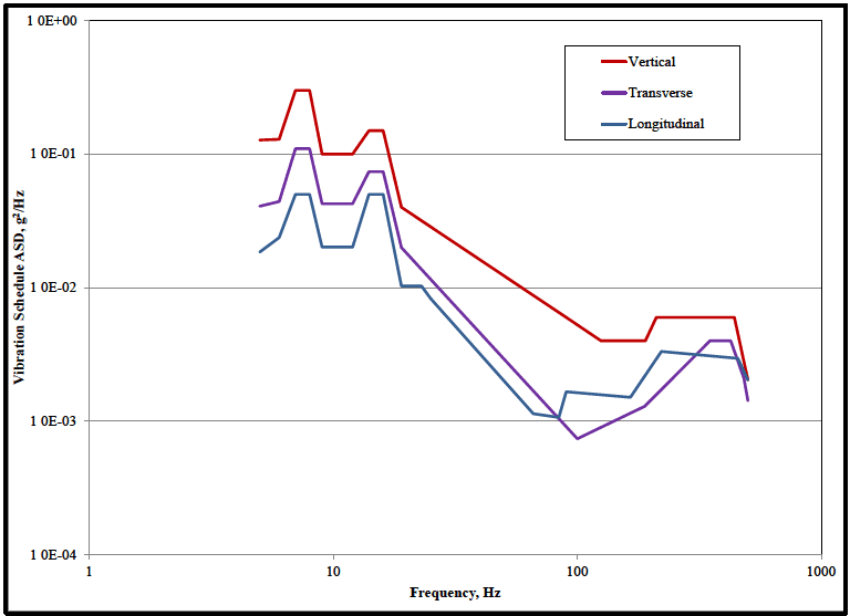
Figure description:
Vibration Schedule ASD vs Frequency (Log-Log Plot Analysis
Vibration Schedule ASD vs Frequency
Legend
- Vertical — color: red; symbol: Thick solid line
- Transverse — color: purple; symbol: Medium solid line with triangle marker
- Longitudinal — color: blue; symbol: Thin solid line with diamond marker
| Frequency (Hz) | Vertical (g²/Hz) | Transverse (g²/Hz) | Longitudinal (g²/Hz) |
|---|---|---|---|
| 5 | 1.30E-01 | 4.10E-02 | 1.90E-02 |
| 6 | 1.30E-01 | 4.50E-02 | 2.50E-02 |
| 7 | 3.00E-01 | 1.10E-01 | 5.00E-02 |
| 8 | 3.00E-01 | 1.10E-01 | 5.00E-02 |
| 9 | 1.00E-01 | 4.20E-02 | 2.10E-02 |
| 12 | 1.00E-01 | 4.20E-02 | 2.10E-02 |
| 14 | 1.50E-01 | 7.50E-02 | 5.00E-02 |
| 16 | 1.50E-01 | 7.50E-02 | 5.00E-02 |
| 19 | 4.00E-02 | 2.00E-02 | 1.00E-02 |
| 25 | null | null | 1.00E-02 |
| 65 | null | null | 1.10E-03 |
| 75 | null | null | 1.10E-03 |
| 85 | null | null | 1.70E-03 |
| 100 | null | 7.50E-04 | null |
| 125 | 4.00E-03 | null | null |
| 170 | null | null | 1.50E-03 |
| 200 | 4.00E-03 | 1.30E-03 | null |
| 220 | 6.00E-03 | null | null |
| 230 | null | null | 3.30E-03 |
| 400 | null | 4.00E-03 | null |
| 450 | 6.00E-03 | 4.00E-03 | 3.00E-03 |
| 500 | 2.00E-03 | 1.40E-03 | 2.00E-03 |
Figure 514.8C-6. - Category 4 - Composite wheeled vehicle vibration exposure.
| Vertical | Transverse | Longitudinal | |||
|---|---|---|---|---|---|
| Frequency, Hz | ASD, g²/Hz | Frequency, Hz | ASD, g²/Hz | Frequency, Hz | ASD, g²/Hz |
| 5 | 0.12765 | 5 | 0.04070 | 5 | 0.01848 |
| 6 | 0.12926 | 6 | 0.04415 | 6 | 0.02373 |
| 7 | 0.30000 | 7 | 0.11000 | 7 | 0.05000 |
| 8 | 0.30000 | 8 | 0.11000 | 8 | 0.05000 |
| 9 | 0.10000 | 9 | 0.04250 | 9 | 0.02016 |
| 12 | 0.10000 | 12 | 0.04250 | 12 | 0.02016 |
| 14 | 0.15000 | 14 | 0.07400 | 14 | 0.05000 |
| 16 | 0.15000 | 16 | 0.07400 | 16 | 0.05000 |
| 19 | 0.04000 | 19 | 0.02000 | 19 | 0.01030 |
| 90 | 0.00600 | 100 | 0.00074 | 23 | 0.01030 |
| 125 | 0.00400 | 189 | 0.00130 | 25 | 0.00833 |
| 190 | 0.00400 | 350 | 0.00400 | 66 | 0.00114 |
| 211 | 0.00600 | 425 | 0.00400 | 84 | 0.00107 |
| 440 | 0.00600 | 482 | 0.00210 | 90 | 0.00167 |
| 500 | 0.00204 | 500 | 0.00142 | 165 | 0.00151 |
| 221 | 0.00333 | ||||
| 455 | 0.00296 | ||||
| 500 | 0.00204 | ||||
| rms = 2.24 g | rms = 1.45 g | rms = 1.32 g | |||
MIL-STD-810H METHOD 514.8, ANNEX C
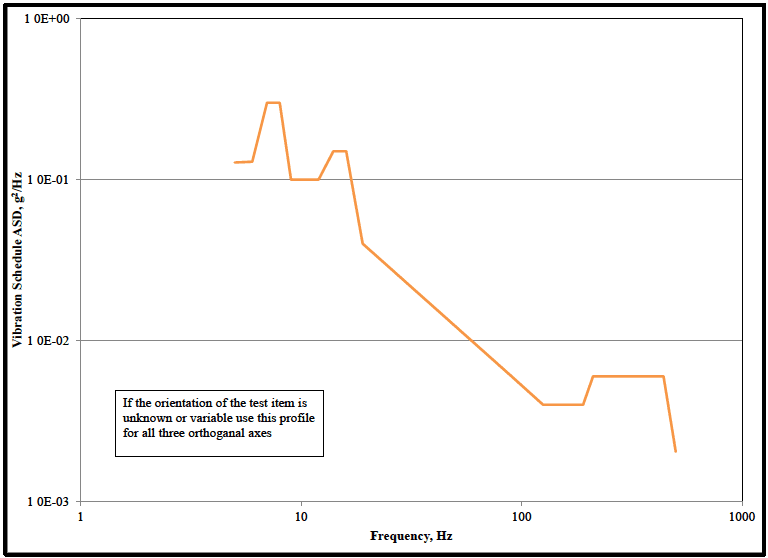
Figure description:
Vibration Schedule ASD vs Frequency
Annotations
- If the orientation of the test item is unknown or variable use this profile for all three orthogonal axes (text_label - position: Center-left in the bottom half of the chart, roughly x=5 to 20, y=0.003 to 0.007)
| Frequency (Hz) | Vibration Schedule ASD (g²/Hz) |
|---|---|
| 5 | 0.13 |
| 6 | 0.13 |
| 7 | 0.30 |
| 8 | 0.30 |
| 9 | 0.10 |
| 12 | 0.10 |
| 14 | 0.15 |
| 16 | 0.15 |
| 19 | 0.04 |
| 130 | 0.004 |
| 200 | 0.004 |
| 220 | 0.006 |
| 450 | 0.006 |
| 500 | 0.002 |
Notes: The chart is a log-log plot. Values are estimated from the provided logarithmic scales on both axes.
Figure 514.8C-7. - Category 4 - Composite wheeled vehicle vibration exposure for unknown orientation.
| Envelope | |
|---|---|
| Frequency, Hz | ASD, g²/Hz |
| 5 | 0.12765 |
| 6 | 0.12926 |
| 7 | 0.30000 |
| 8 | 0.30000 |
| 9 | 0.10000 |
| 12 | 0.10000 |
| 14 | 0.15000 |
| 16 | 0.15000 |
| 19 | 0.04000 |
| 90 | 0.00600 |
| 125 | 0.00400 |
| 190 | 0.00400 |
| 211 | 0.00600 |
| 440 | 0.00600 |
| 500 | 0.00204 |
| rms = 2.24 g | |
2.1.4
Exposure durations. Base durations on the materiel Life Cycle Environment Profile. Figure 514.8C-1 shows the typical field/mission transportation scenario with the most typical vehicles.
- a. Truck transportation over US highways. The exposure duration for common carrier/truck is 60 minutes per 1609 kilometers (1000 miles) of road travel (per axis).
- b. Two-wheeled trailer and wheeled vehicles. The exposure duration for two-wheeled trailer is 32 minutes per 51.5 kilometers (32 miles) traveled (per axis), and the exposure duration for composite wheeled vehicles is 40 minutes per 805 kilometers (500 miles) traveled (per axis).