523.4-2 DEVELOPMENT
2.1 Selecting the Vibro-Acoustic/Temperature Method
After examining requirements documents and applying the tailoring process in Part One of this standard to determine where the vibro-acoustic/temperature environments are anticipated in the life cycle of the materiel, use the following to confirm the need for this method and to place it in sequence with other methods.
523.4-2.1 Background
In order to ensure that the failures occurring in a test are typical of in-service use, it is important to reproduce the service stress distribution. The service stress distribution is the set of stresses in the combinations, levels, and duration imposed by the in-service missions. The procedure reproduces the levels, durations, and combinations of temperature, vibration, and acoustic noise in the same relative proportions as the in-service missions.
2.1.1 Effects of the Vibro-Acoustic/Temperature Environment
Possible effects of a combination of vibration, acoustic noise, and temperature include all effects that these factors can cause separately (see Methods 514, 515, and 520). In addition, increased stress as a result of moisture from thermal change may produce possible effects seen in Methods 501, 502, 503, and 507. The combined vibration, acoustic noise, and temperature environments may interact to produce effects that would not occur in any single environment or a lesser combination of environments. Items in the discussion to follow point to significant effects of mechanisms applicable to this method.
2.1.1.1 Relative Importance of Environmental Stresses
Not all environmental stresses contribute equally to materiel deterioration or failure. Analysis of service-use failures caused by aircraft environmental stress on the store (paragraph 6.1, reference a) has identified the following four most important causes of failure:
- a. loading of the store through captive carriage,
- b. temperature,
- c. vibration, and
- d. moisture.
2.1.1.2 Other Environmental Stresses
Consider the inclusion of other environmental stresses that may be important for particular materiel. In general, it is not appropriate to include comparatively rare occurrences of extreme stress levels that are better quantified in single environment methods described elsewhere in this standard. A general guideline for this determination for an individual stress is that, if a stress has a “fraction of time of occurrence” (FTO) less than 0.1 (10 percent) of the total time specified for the store’s MTBF, the condition may be considered too rare to be included in a test described by this method. In evaluating FTO, consider all in-service use environments and use the more severe of the two. Note that the term FTO is used here in place of the more traditional probability of occurrence. FTO is defined for a level of stress as the ratio of the time the store is under the stress condition divided by the total time of observation, e.g., the store’s mean time between failures. Probability of occurrence relates to the chances a stress event will occur, and may not relate directly to a single specific time interval. FTO can be shown to provide an estimate of the probability distribution of the level of stress and is a more precise term. A simple example of this difference is as follows: If the stress condition is the absolute value of the acceleration at a point in the store that is above 5g’s, the FTO is easily established from an auto-spectral density (ASD) estimate over a specified time interval. This implies a stationary Gaussian time history with zero mean and standard deviation as the square root of the area under the ASD estimate. The probability of occurrence relates to the number of times the 5g level is exceeded, but the total time above 5g may vary from one occurrence to the next, depending on the difference in ASD estimates and on the associated duration of each of the stationary Gaussian ASD estimates.
2.1.1.3 Operation
Operating any materiel item produces stress that can cause failure. In the case of external aircraft stores, operation generally means providing full electrical power that produces thermal, electromagnetic, and electrochemical stress. Duty cycles (on/off), low and high voltage, power ripple, and voltage spikes may also be significant stresses. Even when the stress of operation is negligible, it is necessary to operate the materiel under test to detect the presence of failure. Many failures induced by temperature and some vibration-induced failures are reversible, at least initially. As the test continues, reversible failures tend to become irreversible. Thus, it is important to conduct functional tests while the environmental stresses are present.
MIL-STD-810H
METHOD 523.4
2.1.1.4 Temperature
The most severe temperature shock to internal components may come from powering the materiel when it is cold. In order to induce all the stresses related to temperature in their proper proportion, use a thermal model of the store to predict the temperatures and rates of change at several internal points under service mission profiles.
- a. Ambient temperature. The greatest variations in ambient temperature occur near the surface of the Earth. The low temperature extreme exposure by a store is, in many cases, due to low ambient temperatures immediately preceding flight. This is because there is ample time for temperature soak and there is no internal power dissipation or aerodynamic heating. Hence, it is important to consider on-the-ground temperatures in determining the initial captive flight temperature. The test temperature cycle may need to include a simulated on-the-ground period in order to normalize the temperature for the next simulated mission phase; otherwise an uninterrupted sequence of simulated missions may tend to drive the average internal temperature up or down relative to real missions. NATO STANAG 4370, AECTP 230, and MIL-HDBK-310 (paragraphs 6.1, references b and c) provide ground ambient air temperatures and their probability of occurrence for various regions. The temperatures that are cited in the two documents are those measured for meteorological purposes, and do not include the heating effects of direct sunlight or cooling due to radiation into the night sky. Hence, in determining preflight temperatures, consider the effects of radiation heat transfer, and remember to convert from probability of occurrence to FTO in application.
- b. Aerodynamic heating. During captive flight, the high convective heat transfer rate will cause the surface temperature of an external store to be near that of the boundary layer. The recovery air temperature in the boundary layer depends primarily on the ambient temperature and the speed of flight. The functional dependence is:
M² T₁ = To(1 + r( 1+r(y-1)
where:
- Tr = boundary layer recovery air temperature, °K (°R)
- To = sea level air temperature (standard day), 288.16 °K (518.69 °R)
- θ = ratio temperature at altitude to sea level temperature (standard day) (varies with altitude in two altitude ranges, see Method 514.8, Annex D, Table 514.8D-V)
- r = 0.87, boundary layer temperature recovery factor
- , atmospheric ratio of specific heats
- M = flight Mach number
Since flight at high altitude, where the ambient temperatures are lowest, is usually at higher Mach numbers (>0.80), the low temperatures are generally mitigated by aerodynamic heating. Because of the dominance of boundary layer heat transfer, radiation heat transfer can be neglected in captive flight.
- c. Power dissipation. Although the high heat transfer rate will tend to keep the surface of a store at the boundary layer recovery temperature, internal temperatures may be considerably higher due to power dissipation of electronic equipment. For this reason the duty cycle of the materiel being tested must be tailored to reflect realistic operation and it must be coordinated with the external temperature to achieve a good reproduction of the expected temperatures.
- d. Temperature gradients. The strongest temperature gradients will usually be those associated with powering the materiel when it is cold. Temperature gradients will also occur due to changes in flight speed and altitude that change the surface temperature more rapidly than internal temperatures.
2.1.1.5 Vibration
Vibration may cause mechanical fatigue failure of parts, abrasion due to relative motion, dislodging of loose particles that can cause electrical shorts, and degradation of electronic functions through microphonics and triboelectric noise. Experiments (paragraph 6.1, reference d) and theoretical analysis (paragraph 6.1, reference e) have shown that the relative likelihood of various failure modes change with vibration level. In order to reproduce the service failure modes in proper proportion, it is necessary to test at several levels, keeping the fraction of time (FOT) in each level the same as predicted for the service use. The vibration spectrum may be considered to consist of two parts: the low frequency part that includes those vibrations that can be transmitted from the aircraft, through the store attachments, into the store (this is not the only source of low frequency vibration, but it is the major one), and the high frequency part that is driven almost entirely by pressure fluctuations in the boundary layer acting directly on the surface of the store. Generally, the mechanical impedance of the store attachment is such that the division between low and high frequency is between 100 Hz and 200 Hz.
- a. Low frequency vibration. The low frequency vibration primarily stresses the structure, including brackets, large circuit boards, and electromechanical devices (e.g., gyros, relays). In most cases it is driven by transmission from the aircraft; hence, input excitation through the normal attachment points with a mechanical shaker best reproduces the low frequency vibration. Use Method 514 as a guide. Note that fluctuating aerodynamic forces may also act in the low frequency range. For control surfaces, wings, or other structure with a large area-to-mass ratio, the direct aerodynamic forces may be dominant. For this reason, the low frequency vibration of the test item cannot be regarded as a test of the structural fatigue life for wings, fins, or their attachments. In general, separate tests on components are needed to determine structural fatigue life of these components.
- b. High frequency vibration. Above the frequency at which the store attachments can transmit vibration, the vibration is driven by the boundary layer turbulence (paragraph 6.1, reference f). This vibration does not contribute to failure of the basic structure, but is often a cause of failure in electronics. The characteristics of the pressure fluctuations in the boundary layer are well known (paragraph 6.1, reference g). The significant aspects for external stores are:
- (1) The pressure spectrum is almost flat, out to the highest frequencies to which stores' component parts respond (the -3dB point is about 4000 Hz). Hence, the vibration spectrum of an external store is determined almost entirely by its natural frequency responses.
- (2) The RMS level of the pressure fluctuations, and hence the vibration, is approximately proportional to the dynamic pressure, q, that is a function of flight speed and altitude:
where:
- q = dynamic pressure, kN/m² (lb/ft²)
- ρ0 = sea level atmospheric density, 1.2251x10⁻³ kg/m3 (2.3770x10⁻³ lb sec2/ft4)
- σ = ratio of local atmospheric density to sea level atmospheric density (standard atmosphere) (varies with altitude in two altitude ranges, (see Method 514.8, Table 514.8D-V)
- M = flight Mach number
Modern aircraft flight speed is typically measured in terms of calibrated air speed or Mach number. See Method 514.7, Annex A, paragraph 2.6, and Annex D, Table 514.8D-V (Dynamic pressure calculation) for a more detailed explanation and calculation methods. Determine the proportionality between vibration level at particular points in the store and flight dynamic pressure by flight measurements. If flight data cannot be obtained, use similarity to other stores (paragraph 6.1, reference h), or Method 514.8, Annex D, Table 514.8D-V, and Figures 514.8D-5, -6, and -7 as guidance.
MIL-STD-810H
METHOD 523.4
2.1.1.6 Moisture
Moisture, in conjunction with soluble contaminants, can result in corrosion. In conjunction with electrical power it may result in shorts. Freezing of water in confined spaces may produce mechanical stress. The test cycle should provide for diffusion of water vapor and condensation. The amount of water is generally not important for inducing failures, so humidity need not be controlled in this test. This test is not a substitute for corrosion tests, such as the humidity test (Method 507) or the salt fog test (Method 509).
2.1.1.7 Shock
Shock can cause failure through mechanical stress similar to that induced by vibration. Shocks that are more nearly transient vibrations (many zero crossings), such as aircraft catapult and arrested landing shock may be included in this test. Short duration shocks such as pyrotechnic shocks associated with store or sub-munition launch, flight surface deployment, etc., are generally too difficult to reproduce at the store level. Ensure that these events that are potentially destructive to electronics are accounted for in other analyses and tests (See Method 517, Pyroshock, and Method 516, Shock).
2.1.1.8 Altitude
Barometric pressure is generally not a stress for external stores. However, variation in pressure may enhance the penetration by moisture. Reduced pressure may increase the temperature due to reduced power dissipation and there may be increased electrical arcing. Test separately for resistance to arcing. Moisture penetration will generally take place without pressure variation and, in most cases, the amount of water entrained is not important so long as it is enough to provide internal condensation. Reduced heat transfer may be realized by restricting air circulation rather than reducing ambient pressure. In general, altitude simulation is not needed in this test.
2.1.1.9 Other Environments
Although this method is intended primarily to reproduce the environmental stresses associated with the captive flight of external stores, it can be extended to include other phases of a store's life cycle provided the relative duration of those phases can be related to captive flight. For example, periods of shock and vibration representing transportation and handling have been included in some tests. Do not use environments in this test that are not expected to produce failures randomly distributed in time. For example, corrosive atmospheres and fungal growth are environments in which failures, if any, will occur only after a considerable time lapse. Store ejection shock, sand and dust, and water immersion are examples of environments for which failure either occurs or does not; these failures are associated with the event rather than being distributed in time. These environments are not appropriate for this method. Care is required in deciding which environments to include. For example, consider the case of a store that ejects sub- munitions, flares, chaff, or other items. In this case there will be a series of shock events that may be an important part of the continuing operational store environment. This may also result in open cavities in the store’s external surface resulting in high intensity cavity noise for long periods.
2.1.2 Sequence Among Other Methods
- a. General. Use the anticipated life cycle sequence of events as a general sequence guide (see Part One, paragraph 5.5).
- b. Specific to this method. This method applies to environmental stress occurring in the final phases of the store’s environmental life cycle. When a single test item is subjected to this test and other environmental tests of this standard, perform this test after the tests representing earlier phases of the life cycle, but before tests representing store ejection/launch, free flight, target impact, etc.
2.2 Selecting a Procedure
This method includes one test procedure that may be tailored to many test requirements.
523.4-2.2 General
Military aircraft service use may be described by a set of missions and the relative frequency of occurrence of each mission as illustrated in Table 523.4A-I. Each mission is defined by the type of stores carried and a mission flight profile. The mission flight profile is an idealized mission history that describes altitude, speed, and various events (e.g., air combat, gunfire, refueling) as functions of time. From the mission profiles and climatic data, derive corresponding mission environmental profiles. Use data from instrumented flights in this derivation, if available. Once the mission environmental profiles are derived, they can be combined into a composite mission profile. The composite mission profile is a sequence of environments in which the various stresses and combinations of stresses occur in (approximately) the same proportion as in all of the mission environmental profiles weighted according to their relative frequency of occurrence. The composite mission profile also includes the effects of climatic temperatures according to their relative frequency. However, the composite mission profile must be short enough to be repeated many times (at least five times is recommended) within the expected time-to-failure of the store being tested. This may require that extreme environments (particularly extreme temperatures) not be included, since keeping them in proper proportion might result in too long a composite mission. Typically, the range of stresses included is between the 5th and 95th percentile.
| MISSION TYPE | AIRCRAFT TYPE | % OF SORTIES |
|---|---|---|
| 1. Patrol Mission I | Fighter A | 50 |
| Fighter B | 30 | |
| 2. Patrol Mission II | Fighter A | 20 |
| Fighter B | 20 | |
| 3. Strike Escort Mission | Fighter A | 30 |
| Fighter B | 30 | |
| 4. Strike Mission | Fighter B | 20 |
2.3 Determination of Test Levels and Conditions
Having selected this method, complete the tailoring process by identifying appropriate parameter levels and applicable test conditions and techniques for this procedure. Base these selections on the requirements documents, the Life Cycle Environmental Profile (LCEP), and information provided with this procedure. Consider the following when selecting test levels. Unlike other methods in this standard, this method does not contain any default values for test conditions. The combinations of vibration, acoustics, temperature, and duty-cycle environment are too complex
and the variety of materiel applications too great for such detailed instruction to be given here. Instead, this method provides guidance for writing a test procedure that will be more or less unique to the materiel and test item. Annex A provides a detailed example of the development of test levels and conditions. Before attempting to apply the method, study the example in the Annex. In determination of test levels and conditions, identify the following:
- a. Mission characterization to develop a composite aircraft/store mission profile.
- b. Mission analysis to develop:
- (1) Mission temperature analysis for development of a mission temperature profile over time;
- (2) Mission vibration spectra identification for development of a mission vibration profile over time1;
- (3) Mission operational duty cycle for functional performance of the store over time.
523.4-2.3 Mission Characterization
The first step in developing the composite mission profile is to determine the types of aircraft and mission flight profiles that will employ the store. The mission flight profiles may be described in terms of altitude and Mach number with annotation of events. A tabulated mission phase analysis or mission profile description is shown in Table 523.4A-II. A corresponding graphical representation of this mission is shown on Figure 523.4A-1. The relative frequency of occurrence of the various missions must also be determined. This may be tabulated as shown in
Table 523.4A-I. In determining the relative frequency with which the store will be carried on various missions, it may be necessary to consider some state of hostility. Experience has shown that weapons that would be expended on their first flight in conflict may be subjected to many flights during a time of high international tension in which there is no combat. Choose the most stressful, yet realistic, mix of missions for simulation. Generally, it is not desirable to average together relatively benign missions with relatively stressful ones if a store will experience only one or the other during its service life. For each aircraft type and mission, determine the carriage location of the store to be tested, as well as the location of other stores that may affect it. Stores located ahead of or adjacent to a given store will cause an increase in the turbulence-induced vibration of that store. Ejection of nearby stores may also induce dynamic loads. Also, note any geographic or other conditions that would influence the mission (e.g., a store carried only by carrier-based aircraft will not experience as wide a range of preflight temperatures as one carried by land-based aircraft).
| MISSION PHASE | MACH NUMBER | ALTITUDE (km) | DURATION (min.) | ADDITIONAL FACTORS | DUTY CYCLE OF STORE |
|---|---|---|---|---|---|
| Takeoff & Climb | Catapult Shock? | Off to Ready | |||
| Cruise | Ready | ||||
| Refuel | Ready | ||||
| Ingress | On (Radiate) | ||||
| Attack | Buffet? | Ready | |||
| Return | Ready | ||||
| Refuel | Ready | ||||
| Descend & Land | Landing Shock? | Off |
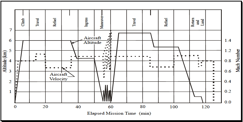
Figure description:
Aircraft Mission Profile Mission Profile Visualization
Aircraft Altitude and Velocity vs. Elapsed Mission Time
Legend
- Aircraft Altitude — color: black; symbol: Solid line
- Aircraft Velocity — color: black; symbol: Dotted line
Annotations
- Climb (text_label - position: x = 2.5, top)
- Travel (text_label - position: x = 9.5, top)
- Refuel (text_label - position: x = 17, top)
- Ingress (text_label - position: x = 42.5, top)
- Maneuver (text_label - position: x = 55, top)
- Travel (text_label - position: x = 72.5, top)
- Refuel (text_label - position: x = 94, top)
- Return and Land (text_label - position: x = 114.5, top)
- Aircraft Altitude (text_label - position: x = 40, y = 5.7)
- Aircraft Velocity (text_label - position: x = 30, y = 3.3)
| Elapsed Mission Time (min) | Aircraft Altitude (km) | Mach Number |
|---|---|---|
| 0 | 0.0 | 0.00 |
| 3 | 3.6 | 0.80 |
| 5 | 6.0 | 0.80 |
| 13 | 6.0 | 0.80 |
| 14 | 6.0 | 0.94 |
| 20 | 6.0 | 0.94 |
| 21 | 6.0 | 0.67 |
| 35 | 6.0 | 0.67 |
| 36 | 5.5 | 0.88 |
| 39 | 4.2 | 0.88 |
| 50 | 4.2 | 0.88 |
| 55 | 0.0 | 0.88 |
| 55.5 | 1.6 | 0.40 |
| 56.5 | 0.0 | 1.10 |
| 57.5 | 1.6 | 0.70 |
| 58.5 | 0.0 | 1.30 |
| 59.5 | 1.6 | 0.90 |
| 60 | 0.0 | 0.88 |
| 65 | 6.7 | 0.88 |
| 83 | 6.7 | 0.88 |
| 85 | 6.7 | 0.70 |
| 87 | 5.3 | 0.70 |
| 100 | 5.3 | 0.70 |
| 102 | 5.3 | 0.90 |
| 103 | 5.3 | 0.90 |
| 113 | 0.7 | 0.90 |
| 115 | 0.7 | 0.90 |
| 116 | 0.7 | 0.80 |
| 118 | 0.7 | 0.80 |
| 119 | 0.0 | 0.80 |
| 125 | 0.0 | 0.80 |
| 126 | 0.0 | 0.00 |
Notes: The Maneuver phase between 50 and 60 minutes features rapid oscillations in both altitude and velocity. Altitude peaks at approximately 1.6 km while velocity (Mach Number peaks at 1.4.)
Figure 523.4A-1. Typical aircraft operational mission profile.
2.4 Test Item Configuration
- a. General. See Part One, paragraph 5.8.
- b. Specific to this method. The configuration of the test item strongly affects test results. Use the anticipated configuration of the materiel in the life cycle profile. As a minimum consider the store captive carry service use environment.
523.4-2.4 Mission Analysis
Rather than deriving store environments such as vibration directly from the mission profiles, first recast the mission profiles in terms of the variables that directly affect the store, but which do not depend on the store’s response.
These variables are initial temperature, recovery air temperature, and dynamic pressure. It is assumed that the store's temperature and vibration are a function of these primary variables.
2.4.1 Mission Temperatures
Standard-day recovery air temperatures may be calculated from the equation in paragraph 2.1.1.4 and Method 514.8, Annex D, Table 514.8D-V, given the flight speed and pressure altitude (h) (standard atmosphere). Table 514.8D-V can also be used to convert various measures of air speed to Mach number. The temperature profile for a single mission type is provided on Figure 523.4A-2. For a composite mission, Figure 523.4A-3 displays the skin temperature versus the elapsed mission time.
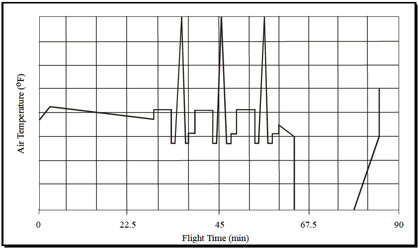
Figure description:
Air Temperature Profile during Flight
Air Temperature vs. Flight Time
| Flight Time (min) | Air Temperature (Relative Units, 0-8) |
|---|---|
| 0 | 3.7 |
| 4.5 | 4.3 |
| 30 | 3.7 |
| 30 | 4.3 |
| 33 | 4.3 |
| 33 | 2.8 |
| 35 | 2.8 |
| 36 | 8 |
| 37 | 2.8 |
| 38.5 | 2.8 |
| 38.5 | 3.2 |
| 40.5 | 3.2 |
| 40.5 | 4.3 |
| 43.5 | 4.3 |
| 43.5 | 2.8 |
| 44.5 | 2.8 |
| 45 | 8 |
| 45.5 | 2.8 |
| 47 | 2.8 |
| 47 | 3.2 |
| 49.5 | 3.2 |
| 49.5 | 4.3 |
| 52.5 | 4.3 |
| 52.5 | 2.8 |
| 53.5 | 2.8 |
| 54 | 8 |
| 54.5 | 2.8 |
| 56.5 | 2.8 |
| 56.5 | 3.2 |
| 58.5 | 3.2 |
| 58.5 | 4.0 |
| 63 | 3.0 |
| 63 | 0 |
| 76.5 | 0 |
| 85.5 | 3.0 |
| 85.5 | 5.0 |
Notes: The y-axis 'Air Temperature (°F' does not have numerical labels; values are estimated relative to the 8 horizontal grid divisions. The x-axis 'Flight Time (min' has major ticks at intervals of 22.5 minutes, with grid lines every 4.5 minutes.))
Figure 523.4A-2. Temperature profile for a single mission type.
MIL-STD-810H METHOD 523.4, ANNEX A
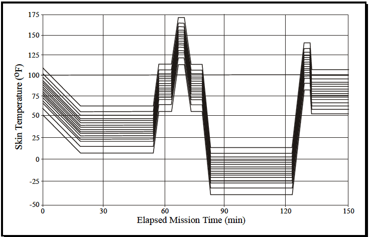
Figure description:
Skin Temperature vs. Elapsed Mission Time
| Elapsed Mission Time (min) | Series 1 (Top) | Series 2 | Series 3 | Series 4 | Series 5 | Series 6 | Series 7 | Series 8 | Series 9 | Series 10 | Series 11 | Series 12 | Series 13 | Series 14 | Series 15 (Bottom) |
|---|---|---|---|---|---|---|---|---|---|---|---|---|---|---|---|
| 0 | 110 | 106 | 102 | 98 | 94 | 90 | 86 | 82 | 78 | 74 | 70 | 66 | 62 | 56 | 50 |
| 19 | 63 | 60 | 56 | 52 | 49 | 46 | 42 | 39 | 35 | 32 | 28 | 24 | 20 | 14 | 7 |
| 54 | 63 | 60 | 56 | 52 | 49 | 46 | 42 | 39 | 35 | 32 | 28 | 24 | 20 | 14 | 7 |
| 57 | 114 | 110 | 106 | 102 | 99 | 96 | 92 | 89 | 85 | 82 | 78 | 74 | 70 | 64 | 55 |
| 64 | 114 | 110 | 106 | 102 | 99 | 96 | 92 | 89 | 85 | 82 | 78 | 74 | 70 | 64 | 55 |
| 67 | 172 | 168 | 164 | 160 | 157 | 154 | 150 | 147 | 143 | 140 | 136 | 132 | 128 | 122 | 113 |
| 71 | 172 | 168 | 164 | 160 | 157 | 154 | 150 | 147 | 143 | 140 | 136 | 132 | 128 | 122 | 113 |
| 74 | 114 | 110 | 106 | 102 | 99 | 96 | 92 | 89 | 85 | 82 | 78 | 74 | 70 | 64 | 55 |
| 78 | 114 | 110 | 106 | 102 | 99 | 96 | 92 | 89 | 85 | 82 | 78 | 74 | 70 | 64 | 55 |
| 82 | 14 | 10 | 6 | 2 | -1 | -4 | -8 | -11 | -15 | -18 | -22 | -26 | -30 | -36 | -40 |
| 123 | 14 | 10 | 6 | 2 | -1 | -4 | -8 | -11 | -15 | -18 | -22 | -26 | -30 | -36 | -40 |
| 128 | 141 | 137 | 133 | 129 | 126 | 123 | 119 | 116 | 112 | 109 | 105 | 101 | 97 | 91 | 83 |
| 131 | 141 | 137 | 133 | 129 | 126 | 123 | 119 | 116 | 112 | 109 | 105 | 101 | 97 | 91 | 83 |
| 133 | 107 | 103 | 99 | 95 | 92 | 89 | 85 | 82 | 78 | 75 | 71 | 67 | 63 | 57 | 52 |
| 150 | 107 | 103 | 99 | 95 | 92 | 89 | 85 | 82 | 78 | 75 | 71 | 67 | 63 | 57 | 52 |
Notes: The graph depicts skin temperature variations for approximately 15 different data series (Series 1-15 over a 150-minute mission. All data series exhibit synchronized temporal behavior, characterized by distinct thermal phases: initial cooling, multiple intermediate plateaus, a sharp temperature spike around 70 minutes, and a sustained cold soak period between 82 and 123 minutes.)
Figure 523.4A-3. Climatic set of temperature profiles for composite mission.
2.4.2 Mission Vibration
- a. Both the frequency spectrum shape and spatial distribution of store vibration in captive flight are almost independent of the flight condition. Exceptions are increased low frequency vibration during buffeting maneuvers and, in some cases, increased high frequency vibration in supersonic flight. In general, boundary layer fluctuating pressures are proportional to the dynamic pressure (q) of the flight condition. The store vibration is the dynamic response of the store to these pressures and is also proportional to q. The vibration spectrum rms level (grms) is proportional to q, and the acceleration spectral density (G) at any frequency is proportional to q². If vibration levels (grmsref, Gref) are defined for a single flight condition (ref), this proportionality can be used to approximate vibration levels throughout the flight envelope as follows:
where: q = dynamic pressure, kN/m² (lb/ft²) grms = spectrum rms vibration level, g G = acceleration spectral density, g²/Hz The area under the G(f) curve is the square of the grms level
-
b. Usually the reference condition is taken to be subsonic carriage on the least stressful aircraft station (wing pylon with no adjacent stores). Using this reference, determine the q versus time profile for each mission and construct a histogram representing the proportion of time the store is at a q level. This summarizes the expected vibration experience of the store. For stores for which measured vibration data are not available, the levels can be estimated by considering similar stores, with tailoring criteria provided in Method 514.8. Paragraph 6.1, reference g is a summary for various air-launched missiles.
-
c. For the missions where the store is carried on stations other than the least stressful station, adjustment factors may be needed. These factors typically account for cases where stores are carried side by side, behind other stores or in other special configurations. Measured data are the best source for these factors. Method 514.8 also provides guidance.
-
d. Vibration of a store is the dynamic response of the store to the fluctuating pressure and aircraft transmitted environments. This is broken down into definitions of the motions of key structural points of the store. The vibration environments of materiel located in the store are the local store vibration responses. The test consists of exciting the store with arbitrary levels of vibration and acoustics, and tailoring these inputs to achieve the defined store responses.
-
e. For the exceptional cases (aircraft buffet, catapult launch, arrested landing, gunfire, etc.), determine vibration/shock level, spectrum, and other characteristics. Quantify the occurrences of the exceptional vibration/shock conditions in terms of duration and mission time, so they can be reproduced in the proper proportions and at the proper times in the test cycle. Measured data are even more important here, but Method 514.8 contains guidance both for interpreting measured data and estimating levels when necessary. Method 519.8 contains guidance on estimating gunfire-induced shock.
2.4.3 Test Temperature Profile
The test temperature profile will be the product of two parts: one that simulates the range and variation of temperature due to the missions, and another that simulates the climatic effects:
- a. To determine the mission simulation part, begin with a sequence of skin temperatures corresponding to a few of the most common mission(s) strung together. Use a sequence that is no longer than one fortieth (1/40) of the store MTBF. It is usually convenient to make it a factor of 24 hours (e.g., 6 hrs or 8 hrs) since the test will be run around-the-clock. Use this skin temperature as an input to the store thermal model and determine the histograms of the internal temperature. These must be the responses after many cycles (the "steady state" responses). Compare these to the histograms for all the missions. Adjust the test sequence to achieve approximate agreement between the temperature histograms, both on the skin and internally. In this adjustment, keep the number and rate of temperature changes roughly the same as in the actual missions. It will usually be necessary to introduce a period of simulated on-the-ground time into the cycle in order that each simulated flight period start with the store at the appropriate uniform temperature. The temperature during the simulated on-the-ground time may be elevated or reduced in order to speed up the stabilization of internal temperatures. This initial temperature will be shifted each cycle to simulate the effect of climatic temperature variation.
- b. Climatic effects are included by repeating the simulated flight cycle with temperatures shifted up or down by offset values that are constant over one cycle, but which differ from cycle to cycle (see Table 523.4A-III). Successive cycles have the temperature raised or lowered by an amount that represents a colder or hotter than standard day. Ensure the number of different offsets is at least eight. The upper bound on the number of offsets is determined by the requirement that the overall cycle must be shorter than one fifth of the MTBF. The value of the N offsets is chosen to be the midpoints of the N equi-probable intervals of the climatic temperature distribution as shown on Figure 523.4A-4. For worldwide, day and night operations, the climatic variation below 10 km is well approximated by a Gaussian distribution; at ground level; the mean is 12 °C and the standard deviation is 15 °C (paragraph 6.1, reference h). (This includes variation of location as well as season.) At altitude, the mean temperature is lower, but the standard deviation is about the same (paragraph 6.1, references h and n) over most of the globe. Near the poles and the equator, the variation at altitude is considerably less (paragraph 6.1, reference o). For eight offsets, the temperatures would be as shown in Table 523.4A-III. Stair-step the sequence of offsets in the test cycle up and down as indicated by the step number. Figure 523.4A-5 displays a climatic set plan where test item skin temperature is a function of elapsed test time. This reduces the duration required between offsets to normalize the store temperature for the next offset. It is desirable to minimize this duration since it does not count in measuring the store MTBF and hence decreases the test efficiency.
MIL-STD-810H
METHOD 523.4, ANNEX A
| STEP | PERCENTILE | OFFSET | GROUND TEMPERATURE |
|---|---|---|---|
| 3 | 6.25 | -30.8°C | -18.8°C (-2°F) |
| 2 | 18.75 | -13.3°C | -1.3°C (30°F) |
| 4 | 31.25 | -7.2°C | 4.8°C (41°F) |
| 1 | 43.75 | -2.4°C | 9.6°C (49°F) |
| 5 | 56.25 | +2.4°C | 14.4°C (58°F) |
| 8 | 68.75 | +7.2°C | 19.2°C (67°F) |
| 6 | 81.25 | +13.3°C | 25.5°C (78°F) |
| 7 | 93.75 | +30.8°C | 43.0°C (109°F) |
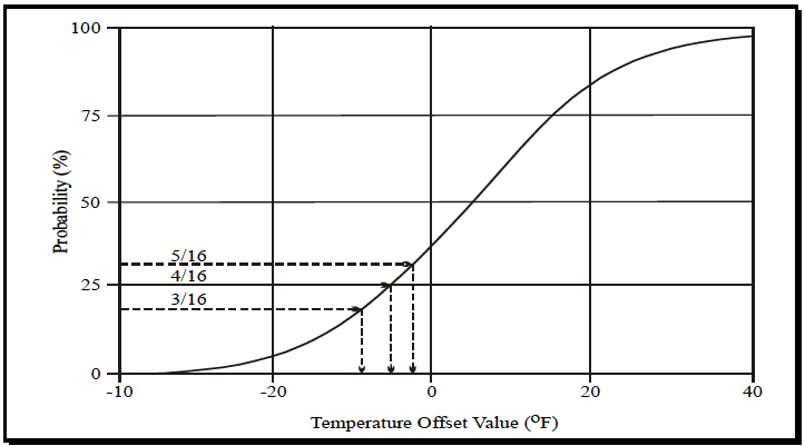
Figure description:
Probability vs. Temperature Offset Value
Annotations
- 5/16 (text_label - position: y = 31.25%)
- 4/16 (text_label - position: y = 25.0%)
- 3/16 (text_label - position: y = 18.75%)
- y = 5/16 reference line (horizontal_line - position: y = 31.25%)
- y = 4/16 reference line (horizontal_line - position: y = 25.0%)
- y = 3/16 reference line (horizontal_line - position: y = 18.75%)
- x-intercept for y = 5/16 (vertical_line - position: x ≈ -2.5)
- x-intercept for y = 4/16 (vertical_line - position: x ≈ -5.0)
- x-intercept for y = 3/16 (vertical_line - position: x ≈ -9.0)
| Temperature Offset Value (°F) | Probability (%) |
|---|---|
| -40 | 0.0 |
| -30 | 1.5 |
| -20 | 5.0 |
| -10 | 16.5 |
| -9.0 | 18.75 |
| -5.0 | 25.0 |
| -2.5 | 31.25 |
| 0 | 38.0 |
| 5 | 50.0 |
| 10 | 65.0 |
| 15 | 77.0 |
| 20 | 85.0 |
| 25 | 92.0 |
| 30 | 95.0 |
| 35 | 97.0 |
| 40 | 98.5 |
Notes: The chart represents a cumulative probability distribution of temperature offset values. Specific annotations highlight the probabilities of 3/16, 4/16, and 5/16 and their corresponding temperature offset values.
Figure 523.4A-4. Selection of equi-probable temperatures from the cumulative distribution of climatic temperatures.
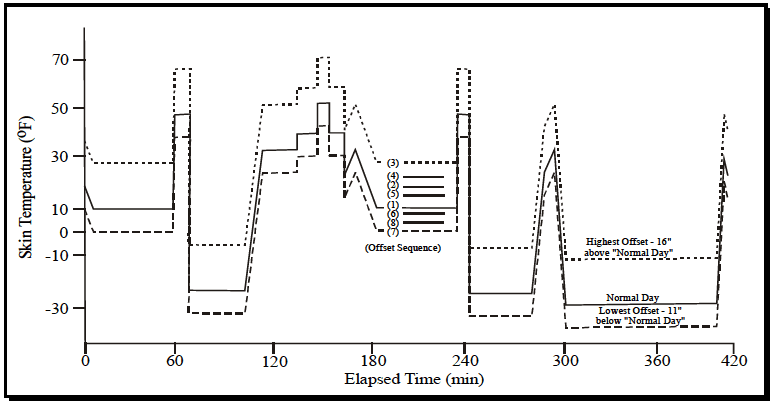
Figure description:
Skin Temperature Profile
Skin Temperature (°F vs Elapsed Time (min
Legend
- Normal Day — color: black; symbol: Solid line
- Highest Offset — color: black; symbol: Dotted line
- Lowest Offset — color: black; symbol: Dashed line
Annotations
- (Offset Sequence: (3, (4, (2, (5, (1, (6, (8, (7 (text_label - position: Centered around x = 200, y = 10))))))))))
- Highest Offset - 16" above "Normal Day" (text_label - position: Right side, near y = -10)
- Normal Day (text_label - position: Right side, near y = -25)
- Lowest Offset - 11" below "Normal Day" (text_label - position: Right side, near y = -35)
| Elapsed Time (min) | Normal Day (°F) | Highest Offset (+16°F) | Lowest Offset (-11°F) |
|---|---|---|---|
| 0 | 18 | 34 | 7 |
| 10 | 10 | 26 | -1 |
| 60 | 10 | 26 | -1 |
| 60 | 48 | 64 | 37 |
| 65 | 48 | 64 | 37 |
| 65 | 38 | 54 | 27 |
| 70 | 38 | 54 | 27 |
| 70 | -24 | -8 | -35 |
| 105 | -24 | -8 | -35 |
| 115 | 33 | 49 | 22 |
| 135 | 33 | 49 | 22 |
| 145 | 40 | 56 | 29 |
| 155 | 52 | 68 | 41 |
| 165 | 40 | 56 | 29 |
| 170 | 22 | 38 | 11 |
| 175 | 33 | 49 | 22 |
| 185 | 11 | 27 | 0 |
| 235 | 11 | 27 | 0 |
| 235 | 48 | 64 | 37 |
| 240 | 48 | 64 | 37 |
| 240 | 38 | 54 | 27 |
| 245 | 38 | 54 | 27 |
| 245 | -25 | -9 | -36 |
| 280 | -25 | -9 | -36 |
| 295 | 33 | 49 | 22 |
| 300 | -29 | -13 | -40 |
| 405 | -29 | -13 | -40 |
| 410 | 32 | 48 | 21 |
| 415 | 23 | 39 | 12 |
Notes: The chart shows a sequence of skin temperature changes over time. The 'Normal Day' line serves as a baseline, with 'Highest' and 'Lowest' offset lines plotted at +16°F and -11°F respectively. Intermediate offset lines are partially visible in some segments and are identified by the '(Offset Sequence' labels (1 through (8 in the middle of the plot.)))
Figure 523.4A-5. Climatic set plan showing offset sequences.
2.4.4 Test Vibration Profile
Ensure the test vibration profile produces the same histogram of store response levels as that derived from the mission analysis. Analyses assuming power function fatigue damage indicate that three to five different vibration levels are usually enough (paragraph 6.1, reference p). Use the same mission sequence used for the initial temperature cycle to generate a vibration level test cycle. This can then be adjusted to achieve the correct overall histogram. Maintain correlation between vibration and temperature (usually high vibration level goes with high temperature) as in the actual missions. Insert the exceptional vibration events into the test cycle with proportionate duration, and in realistic combination with the temperature and the straight and level vibration. Usually it is desirable to test the function of the store under the more severe part of the test environment, since that is the most likely to reveal reversible failures. In service, high levels of vibration, such as those due to buffet, usually occur over several very short time intervals, on the order of a few seconds. It may be desirable to conjoin all the high level vibration corresponding to a few mission-hours into a single interval in order to allow time for a complete test of the store's function during the high level vibration. Figure 523.4A-6 displays dynamic pressure, q, in terms of absolute pressure, Pa, versus elapsed mission time for a composite mission.
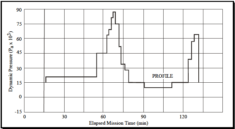
Figure description:
Dynamic Pressure Profile vs. Elapsed Mission Time
Annotations
- PROFILE (text_label - position: x = 100, y = 23)
| Elapsed Mission Time (min) | Dynamic Pressure (Pa x 10³) |
|---|---|
| 15 | 0 |
| 15 | 21 |
| 55 | 21 |
| 55 | 45 |
| 62 | 45 |
| 62 | 64 |
| 64 | 64 |
| 64 | 69 |
| 66 | 69 |
| 66 | 81 |
| 68 | 81 |
| 68 | 87 |
| 70 | 87 |
| 70 | 75 |
| 72 | 75 |
| 72 | 52 |
| 74 | 52 |
| 74 | 34 |
| 76 | 34 |
| 76 | 28 |
| 79 | 28 |
| 79 | 15 |
| 90 | 15 |
| 90 | 10 |
| 111 | 10 |
| 111 | 15 |
| 123 | 15 |
| 123 | 39 |
| 125 | 39 |
| 125 | 57 |
| 127 | 57 |
| 127 | 64 |
| 131 | 64 |
| 131 | 15 |
Notes: The chart is a step plot representing dynamic pressure over time. The values for time and pressure are estimated from the provided graphical representation, specifically using the grid lines which occur every 10 minutes on the x-axis and every 15 units (x 10³ on the y-axis.)
Figure 523.4A-6. Dynamic pressure, q, profile for composite mission.
2.4.5 Operational Duty Cycle
Consider the operational duty cycle of the store in the temperature test design since power dissipation is a source of heat. Additionally, arrange it to allow functional test of the store during stressful parts of the cycle, as well as benign parts. If possible, test the store at low and high temperature extremes, during or immediately after high level vibration and at the beginning of each cycle.