528.1-2 PROCEDURE
528.1-2 ACQUISITION REQUIREMENTS
Acquisition documents should specify the following:
- a. Title, number, and date of the method.
- b. Reporting requirements, including requirements for Notification of Test, Equipment Test Plan, and/or Test Report (see paragraphs 4.1, 5.1.2.5.1, and 5.1.2.5.2 in the front part of this Method).
- c. Identification of component compliance on component drawing, in Test Report, or on label plate (see paragraph 4.2).
- d. Disposition of tested equipment and related equipment (see paragraph 4.3 in the front part of this Method).
- e. Type(s) of vibration required (see paragraphs 5.1 and 5.2 in the front part of this Method).
- f. Type I:
- (1) How the equipment will be operated after the test to demonstrate the machinery or equipment has no damage from the test, including acceptable operational degradations (see paragraphs 5.1.1 and 5.1.2.4.1 in the front part of this Method).
- (2) Whether the test engineer needs concurrence of the procuring agency for determination of major vs. minor failures before continuing testing (see paragraph 5.1.1 in the front part of this Method).
- (3) Whether measurement transducer locations need to be approved by the procuring agency for Type I testing (see paragraph 5.1.2.2) in the front part of this Method).
- (4) Methods of mounting equipment for test (see paragraph 5.1.2.3.4 in the front part of this Method).
- (5) Whether internal mounts should be installed for all, a specific part, or none of the test (see paragraph 5.1.2.3.5 in the front part of this Method).
- (6) How the test item will be energized or operated during Type I vibration tests (e.g., pressure, flow rate, voltage current, and cycling of principal functions during testing), including acceptable operational degradations (see paragraphs 5.1.1 and 5.1.2.4.1 in the front part of this Method).
- (7) When required, the maximum test frequencies (see paragraph 5.1.2.4.4 in the front part of this Method)
MIL-STD-810H METHOD
528.1-2 DISTRIBUTION OF CLIMATIC DESIGN TYPES
There are four climatic design types: Hot (A1 and B3), Basic (A2, B1, B2, and C1), Cold (C2), and Severe Cold (C3). Figure 1 shows land areas where the four climatic design types apply. Discussion of the delimitation of the climatic conditions (paragraph 2.2) is included to permit proper interpretation and use of the map. The primary basis for delimiting the climatic conditions is temperature; secondary consideration is given to humidity conditions.
528.1-2 MIL-HDBK-310
MIL-HDBK-310, “Global Climatic Data for Developing Military Products,” includes extensive information regarding extreme natural environments. Consult MIL-HDBK-310 directly for more specific details.
The following data table was extracted from a publication by Dr. Paul Krause and Ms. Kathleen Flood of the Army Topographic Engineering Center. The publication is: Krause, P.F. and K.L. Flood. 1997. Weather and Climate Extremes (Technical Report TEC-0099). Alexandria, VA: U.S. Army Topographic Engineering Center.
Table A-I. Weather & Climatic Extremes – Brief Summary.
| Temperature Extremes | |||
|---|---|---|---|
| Lowest | °C (°F) | Location | Date |
| North America (excluding Greenland) | -63 (-81.4) | Snag, Yukon Territory | 3 February 1947 |
| US Coolest Summer Average | 2.2 (36) | Barrow, AK | 1941-1970 |
| US Lowest Annual Mean | -12.8 (9) | Barrow, AK | 1941-1970 |
| US | -62.1 (-79.8) | Prospect Creek, AK | 23 January 1971 |
| US (excluding Alaska) | -56.5 (-69.7) | Rogers Pass, MT | 20 January 1954 |
| US Coldest Winter Average | -26.7 (-16) | Barter Island, AK | 1941-1970 |
| CA Lowest Annual Mean | -19.4 (-3) | Eureka, NW Territories | 1947-1980 |
| North America - Mean (Month) (excluding Greenland) | -47.8 (-54) | Eureka, NW Territories | February 1979 |
| Greenland | -66.1 (-87) | Northice | 9 January 1954 |
| Europe | -55 (-67) | Ust'Shchugor, Russia | 15 Year Period |
| Northern Hemisphere | -67.8 (-90) | Verkhoyansk & Oimekon, Russia | 5 & 7 Feb 1892, and 6 Feb 1933 |
| Africa | -23.9 (-11) | Ifrane, Morocco | 11 February 1935 |
| South America | 32.8 (-27) | Sarmiento, Argentina | 1 June 1907 |
| Australia | -23 (-9.4) | Charlotte Pass, New South Wales | 29 June 1994 |
| Antarctica Mean Monthly | -73.2 (-99.8) | Plateau Station | July 1968 |
| Antarctica Annual Mean | -57.2 (-71) | Sovietskaya | 1957 & 1958 |
| World | -88.9 (-128) | Vostok, Antarctica | 21 July 1983 |
MIL-STD-810H
PART THREE ANNEX A
Table A-I. Weather & Climatic Extremes – Brief Summary – continued
| Temperature Extremes | |||
|---|---|---|---|
| Highest | °C (°F) | Location | Date |
| US Winter Average | 22.8 (73) | Honolulu, HI | 1941 to 1970 |
| Western Hemisphere | 56.7 (134) | Greenland Ranch, CA | 10 July 1913 |
| Western Hemisphere Summer Average | 37 (98) | Death Valley, CA | 1941-1970 |
| CA | 45 (113) | Midale & Yellow Grass, Saskatchewan | 5 July 1937 |
| Europe | 50 (122) | Seville, Spain | 4 August 1881 |
| World | 56.7 (134) | Greenland Ranch, CA | 10 July 1913 |
| Asia | 53.9 (129) | Tirat Tsvi, Israel | 21 June 1942 |
| World Annual Mean | 34.4 (94) | Dallol, Ethiopia | Oct 1960 to Nov 1966 |
| Australia | 50.7 (123.3) | Oodnadatta, South Australia | 2 Jan 1960 |
| South America | 48.9 (120) | Rivadavia, Argentina | 11 December 1905 |
| South Pole | -13.6 (7.5) | South Pole | 27 December 1978 |
| Antarctica | 15 (59) | Vanda Station | 5 January 1974 |
| Miscellaneous | |||
| US Largest 24-hour Temperature Fall | 56 (100) | Browning, MT | 23 & 24 January 1916 |
| Western Hemisphere -Difference Between Lowest & Highest Recorded Temperatures | 98.3 (177) | Mayo, Yukon Territory, CA | Unknown |
| US Largest 2-minute Temperature Rise | 27.2 (49) | Spearfish, SD | 22 January 1943 |
| Eastern Hemisphere -Difference Between Lowest & Highest Recorded Temperatures | 101.8 (183.2) | Verkhoyansk, Russia | Unknown |
| Mean Annual Temperature Range | 81.1 (146) | Eastern Sayan Region, Russia | Unknown |
| Australia Longest Hot Spell | =/> 37.8 (100) | Marble Bar | 30 October 1923 to 7 April 1924 (162 consecutive days) |
MIL-STD-810H PART THREE ANNEX A
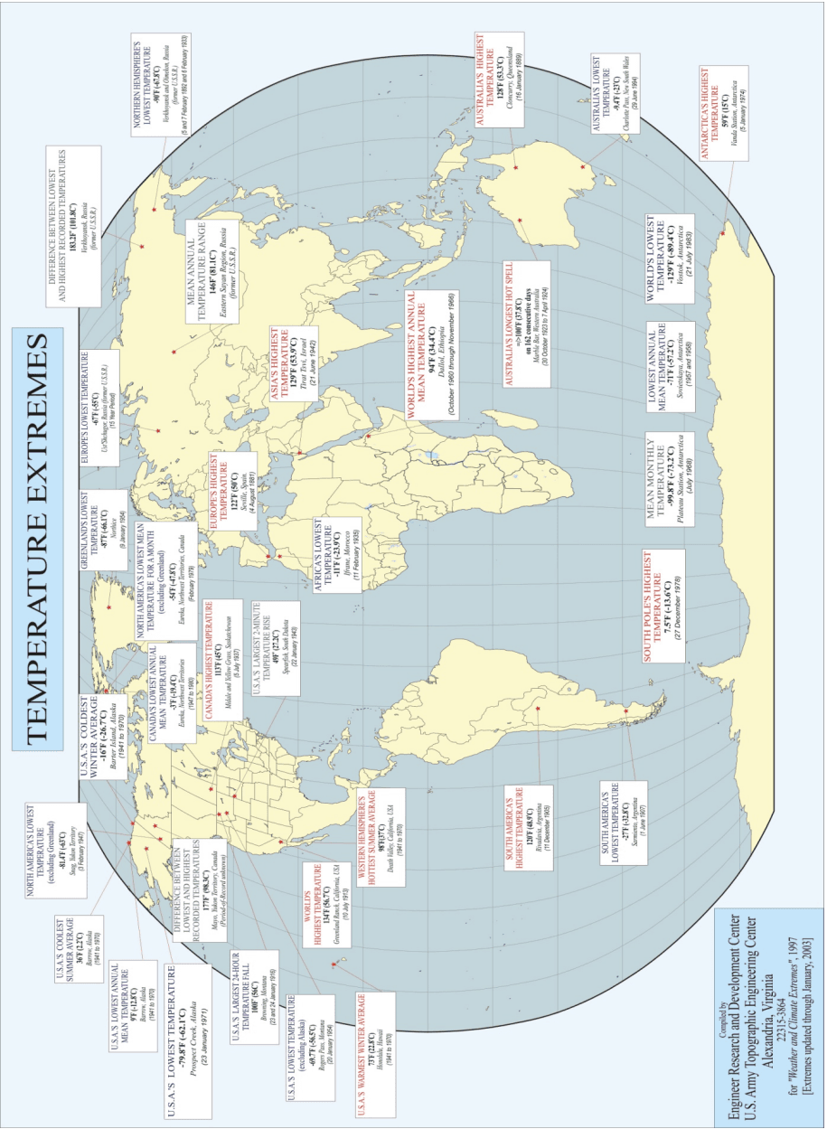
Figure description:
TEMPERATURE EXTREMES
TEMPERATURE EXTREMES
| Extreme Description | Temperature (°F) | Temperature (°C) | Location | Date / Period |
|---|---|---|---|---|
| North America's Lowest Temperature (excluding Greenland) | -81.4°F | -63°C | Snag, Yukon Territory | 3 February 1947 |
| U.S.A.'s Coolest Summer Average | 36°F | 2.2°C | Barrow, Alaska | 1941 to 1970 |
| U.S.A.'s Lowest Annual Mean Temperature | 9°F | -12.8°C | Barrow, Alaska | 1941 to 1970 |
| U.S.A.'s Lowest Temperature | -79.8°F | -62.1°C | Prospect Creek, Alaska | 23 January 1971 |
| U.S.A.'s Coldest Winter Average | -16°F | -26.7°C | Barter Island, Alaska | 1941 to 1970 |
| Canada's Lowest Annual Mean Temperature | -3°F | -19.4°C | Eureka, Northwest Territories | 1947 to 1980 |
| Difference Between Lowest and Highest Recorded Temperatures | 177°F | 98.3°C | Mayo, Yukon Territory, Canada | Period-of-Record unknown |
| North America's Lowest Mean Temperature for a Month (excluding Greenland) | -54°F | -47.8°C | Eureka, Northwest Territories, Canada | February 1979 |
| Canada's Highest Temperature | 113°F | 45°C | Midale and Yellow Grass, Saskatchewan | 5 July 1937 |
| U.S.A.'s Largest 24-Hour Temperature Fall | 100°F | 56°C | Browning, Montana | 23 and 24 January 1916 |
| U.S.A.'s Lowest Temperature (excluding Alaska) | -69.7°F | -56.5°C | Rogers Pass, Montana | 20 January 1954 |
| U.S.A.'s Largest 2-Minute Temperature Rise | 49°F | 27.2°C | Spearfish, South Dakota | 22 January 1943 |
| World's Highest Temperature | 134°F | 56.7°C | Greenland Ranch, California, USA | 10 July 1913 |
| U.S.A.'s Warmest Winter Average | 73°F | 22.8°C | Honolulu, Hawaii | 1941 to 1970 |
| Western Hemisphere's Hottest Summer Average | 98°F | 37°C | Death Valley, California, USA | 1941 to 1970 |
| Greenland's Lowest Temperature | -87°F | -66.1°C | Northice | 9 January 1954 |
| Europe's Lowest Temperature | -67°F | -55°C | Ust'Shchugor, Russia (former U.S.S.R.) | 15 Year Period |
| Europe's Highest Temperature | 122°F | 50°C | Seville, Spain | 4 August 1881 |
| Africa's Lowest Temperature | -11°F | -23.9°C | Ifrane, Morocco | 11 February 1935 |
| South America's Highest Temperature | 120°F | 48.9°C | Rivadavia, Argentina | 11 December 1905 |
| South America's Lowest Temperature | -27°F | -32.8°C | Sarmiento, Argentina | 1 June 1907 |
| Difference Between Lowest and Highest Recorded Temperatures | 183.2°F | 101.8°C | Verkhoyansk, Russia (former U.S.S.R.) | null |
| Northern Hemisphere's Lowest Temperature | -90°F | -67.8°C | Verkhoyansk and Oimekon, Russia (former U.S.S.R.) | 5 and 7 February 1892 and 6 February 1933 |
| Mean Annual Temperature Range | 146°F | 81.1°C | Eastern Sayan Region, Russia (former U.S.S.R.) | null |
| Asia's Highest Temperature | 129°F | 53.9°C | Tirat Tsvi, Israel | 21 June 1942 |
| World's Highest Annual Mean Temperature | 94°F | 34.4°C | Dallol, Ethiopia | October 1960 through November 1966 |
| Australia's Highest Temperature | 128°F | 53.3°C | Cloncurry, Queensland | 16 January 1889 |
| Australia's Longest Hot Spell | >=100°F | 37.8°C | Marble Bar, Western Australia | 30 October 1923 to 7 April 1924 (on 162 consecutive days) |
| Australia's Lowest Temperature | -9.4°F | -23°C | Charlotte Pass, New South Wales | 29 June 1994 |
| South Pole's Highest Temperature | 7.5°F | -13.6°C | null | 27 December 1978 |
| Mean Monthly Temperature | -99.8°F | -73.2°C | Plateau Station, Antarctica | July 1968 |
| Lowest Annual Mean Temperature | -71°F | -57.2°C | Sovietskaya, Antarctica | 1957 and 1958 |
| World's Lowest Temperature | -129°F | -89.4°C | Vostok, Antarctica | 21 July 1983 |
| Antarctica's Highest Temperature | 59°F | 15°C | Vanda Station, Antarctica | 5 January 1974 |
Source: Compiled by Engineer Research and Development Center, U.S. Army Topographic Engineering Center, Alexandria, Virginia, for "Weather and Climate Extremes", 1997 [Extremes updated through January, 2003 Notes: The map displays various temperature extremes recorded globally, including record highs and lows, largest changes, and highest/lowest averages.
MIL-STD-810H
PART THREE ANNEX A
Table A-II Precipitation extremes
| Greatest | Cm (in) | Location | Date |
|---|---|---|---|
| Possibly World 1-Minute Rainfall | 3.12 (1.5) | Barot, Guadeloupe, West Indies | 26 November 1970 |
| World 1-Minute Rainfall | 3.1 (1.23) | Unionville, MD | 4 July 1956 |
| World 20-Minute Rainfall | 20.6 (8.10) | Curtea-de-Arges, Romania | 7 July 1889 |
| World 42-Minute Rainfall | 30.5 (12) | Holt, MO | 23 June 1947 |
| Possibly World 60-Minute Rainfall | 41.1 (15.78) | Muduocaidang, Nei Monggol, China | 1 August 1977 |
| World 12-Hour Rainfall | 117 (46) | Grand Ilet, La R'eunion Island | 26 January 1980 |
| Canada 24-Hour Rainfall | 49 (19.3) | Ucluelet Brynnor Mines, BC | 6 October 1967 |
| US 24-Hour Rainfall | 109 (43) | Alvin, TX | 25-26 July 1979 |
| Northern Hemisphere 24-Hour Rainfall | 125 (49.2) | Paishih, Taiwan | 10-11 September 1963 |
| Australia 24-Hour Rainfall | 114 (44.9) | Bellenden Ker, Queensland | 4 January 1979 |
| World 24-Hour Rainfall | 182.5 (72) | Foc-Foc, La R'eunion Island | 7-8 January 1966 |
| World 5-Day Rainfall | 430 (169.3) | Commerson, La Réunion Island | 23-28 January 1980 |
| World 1-Month Rainfall | 930 (366) | Cherrapunji, India | July 1861 |
| US Rainfall (12-Month) | 1877 (739) | Kukui, Maui, HI | December 1981 to December 1982 |
| World Rainfall (12-Month) | 2647 (1042) | Cherrapunji, India | August 1860 to July 1861 |
| North America Average Yearly Precipitation | 650 (256) | Henderson Lake, British Columbia, CA | 14-year Period |
| Australia Average Yearly Precipitation | 864 (340.16) | Bellenden Ker, Queensland | 9-year Period |
| South America Average Yearly Precipitation | 899 (354) | Quibdo, Columbia | 1931 to 1946 |
| Africa Average Yearly Precipitation | 1029 (405) | Debundscha, Cameroon | 32-year Period |
| Europe Average Yearly Precipitation | 465 (183) | Crkvice (former Yugoslavia) | 22-year Period |
| US (& Possibly World) Average Yearly Precipitation | 1168 (460) | Mount Waialeale, Kauai, HI | 1931 to 1960 |
| Asia (& Possibly World) Average Yearly Precipitation | 1187.3 (467.4) | Mawsynram, India | 1941 to 1979 |
| SA & Possibly World Average Yearly Precipitation | 1330 (523.6) | Lloro, Columbia | 1932 to 1960 |
MIL-STD-810H
PART THREE ANNEX A
Table A-II Precipitation extremes – continued
| Snowfall | Cm (in) | Location | Date |
|---|---|---|---|
| France | 172 (67.7) | Bessans | 5-6 April 1969 |
| North America 24-hour | 193 (76) | Silver Lake, CO | 14-15 April 1921 |
| US Extreme Event | 195.6 (77) (Not Official) | Montague Township, NY | 11-12 January 1997 |
| North America - One Storm | 480 (189) | Mt Shasta Ski Bowl, CA | 13-19 February 1959 |
| North America - One Season | 2896 (1140) | Mt Baker Ski Area, WA | 1998 to 1999 |
| Canada One Season | 2446.5 (963) | Revelstoke, Mt Copeland, BC | 1971-1972 |
| North America - Depth of Snow on Ground | 1145.5 (451) | Tamarack, CA | 11 March 1911 |
| Lowest | |||
| Cm (in) | Location | Date | |
| North America Average Yearly Precipitation | 3 (1.2) | Bataques, Mexico | 14-year Period |
| Western Hemisphere Average Yearly Precipitation | 4.1 (1.63) | Death Valley, CA | 1911 to 1953 |
| Europe Average Yearly Precipitation | 16.3 (6.4) | Astrakhan, Russia | 25-year Period |
| Africa Average Yearly Precipitation | <0.25 (<0.1) | Wadi Halfa, Sudan | 39-year Period |
| Asia Average Yearly Precipitation | 4.6 (1.8) | Aden, South Yemen | 50-year Period |
| Australia Average Yearly Precipitation | 10 (4.05) | Troudaninna, South Australia | 42-year Period |
| World Average Yearly Precipitation | 0.08 (0.03) | Arica, Chile | 59-year Period |
| Hailstones | |||
| Size | Location | Date | |
| Canada - Heaviest | 290 g (10.23) | Cedoux, Saskatchewan | 27 August 1973 |
| US Largest Circumference | 47.6 cm (18.75 in) | Aurora, Nebraska | 22 June 2003 |
| World - Heaviest | 1.02 kg (2.25 lb) | Gopalganj District, Bangladesh | 14 April 1986 |
| Miscellaneous | |||
| Unit | Location | Date | |
| US - Longest Dry Period | 767 Days | Bagdad, CA | 3 October 1912 to 8 November 1914 |
| Years Without Rain | >14 Consecutive | Arica, Chile | October 1903 to January 1918 |
| Greatest Average Number of Days Per Year With Rain | 325 | Bahia Felix, Chile | |
| Africa Greatest Average Variability of Annual Precipitation | 191 cm (75 cm) | Debundscha, Cameroon | |
| Relative Variability of Annual Precipitation | 94 percent | Themed, Israel | 1921 to 1947 |
| Relative Variability of Annual Precipitation | 108 percent | Lhasa, Tibet | 1935 to 1939 |
MIL-STD-810H
PART THREE ANNEX A
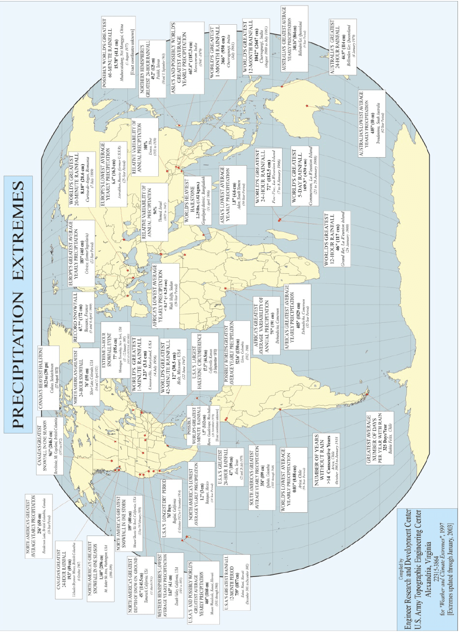
Figure description:
PRECIPITATION EXTREMES
World Precipitation Extremes Map
Annotations
- Thompson Pass, Alaska: Not an official record (text_label - position: Alaska)
- Barot, Guadeloupe: Exact coordinates unknown (text_label - position: Guadeloupe)
- Muduoxiang, China: Exact coordinates unknown (text_label - position: China)
| Location | Record Type | Value | Date / Period |
|---|---|---|---|
| Henderson Lake, British Columbia, Canada | North America's Greatest Average Yearly Precipitation | 256" (650 cm) | 14-Year Period |
| Revelstoke, Mt. Copeland, British Columbia, Canada | Canada's Greatest Snowfall in One Season | 963" (2446.5 cm) | 1971 to 1972 |
| Cedoux, Saskatchewan, Canada | Canada's Heaviest Hailstone | 10.23 oz (290 gm) | 27 August 1973 |
| Ucluelet Brynnor Mines, British Columbia, Canada | Canada's Greatest 24-Hour Rainfall | 19.3" (49 cm) | 6 October 1967 |
| Mt. Baker Ski Area, Washington, USA | North America's Greatest Snowfall in One Season | 1,140" (2896 cm) | 1998-1999 |
| Mount Shasta Ski Bowl, California, USA | North America's Greatest Snowfall in One Storm | 189" (480 cm) | 13 to 19 February 1959 |
| Silver Lake, Colorado, USA | North America's Greatest 24-Hour Snowfall | 76" (193 cm) | 14 to 15 April 1921 |
| Thompson Pass, Alaska, USA | Extreme 24-Hour Snowfall Event (NOT AN OFFICIAL RECORD) | 77" (195.6 cm) | 6 and 7 December 1999 |
| Tamarack, California, USA | North America's Greatest Depth of Snow on Ground | 451" (1145.5 cm) | 11 March 1911 |
| Bagdad, California, USA | U.S.A.'s Longest Dry Period | 767 Days | 3 October 1912 to 8 November 1914 |
| Death Valley, California, USA | Western Hemisphere's Lowest Average Yearly Precipitation | 1.63" (4.1 cm) | 1911 to 1953 |
| Unionville, Maryland, USA | World's Greatest 1-Minute Rainfall | 1.23" (3.1 cm) | 4 July 1956 |
| Holt, Missouri, USA | World's Greatest 12-Minute Rainfall | 12" (30.5 cm) | 22 June 1947 |
| Kukui, Maui, Hawaii, USA | U.S.A.'s Greatest Rainfall 12-Month Period | 739" (1877 cm) | December 1981 to December 1982 |
| Mt. Waialeale, Kauai, Hawaii, USA | U.S.A.'s and Possibly World's Greatest Average Yearly Precipitation | 460" (1168 cm) | 1931 through 1960 |
| Bataques, Mexico | North America's Lowest Average Yearly Precipitation | 1.2" (3 cm) | 14-Year Period |
| Barot, Guadeloupe, West Indies | Possibly World's Greatest 1-Minute Rainfall | 1.5" (3.8 cm) | [Exact coordinates unknown |
| Coffeyville, Kansas, USA | U.S.A.'s Largest Hailstone Circumference | 17.5" (44.5 cm) | 3 September 1970 |
| Alvin, Texas, USA | U.S.A.'s Greatest 24-Hour Rainfall | 43" (109 cm) | 25 and 26 July 1979 |
| Quibdó, Colombia | South America's Greatest Average Yearly Precipitation | 354" (899 cm) | 1931 through 1946 |
| Lloró, Colombia | Possibly World's Greatest Average Yearly Precipitation | 523.6" (1330 cm) | 1932 - 1960 |
| Arica, Chile | World's Lowest Average Yearly Precipitation | 0.03" (0.08 cm) | 59-Year Period |
| Iquique, Chile | Number of Years Without Rain | >14 Consecutive Years | October 1903 to January 1918 |
| Bahía Félix, Chile | Greatest Average Number of Days Per Year With Rain | 325 Days/Year | null |
| Bessans, France | Record Snowfall | 67.7" (172 cm) | 5 and 6 April 1959 |
| Crkvice (formerly Yugoslavia) | Europe's Greatest Average Yearly Precipitation | 183" (465 cm) | 22-Year Period |
| Curtea-de-Arges, Romania | World's Greatest 20-Minute Rainfall | 8.10" (20.6 cm) | 7 July 1889 |
| Astrakhan, Russia (former U.S.S.R.) | Europe's Lowest Average Yearly Precipitation | 6.4" (16.3 cm) | 25-Year Period |
| Themed, Israel | Relative Variability of Annual Precipitation | 94% | 1921 to 1947 |
| Wadi Halfa, Sudan | Africa's Lowest Average Yearly Precipitation | <0.1" (<0.25 cm) | 39-Year Period |
| Debundscha, Cameroon | Africa's Greatest Average Variability of Annual Precipitation | 75% (191 cm) | null |
| Debundscha, Cameroon | Africa's Greatest Average Yearly Precipitation | 405" (1029 cm) | 32-Year Period |
| Grand Îlet, La Réunion Island | World's Greatest 12-Hour Rainfall | 46" (117 cm) | 26 January 1980 |
| Foc-Foc, La Réunion Island | World's Greatest 24-Hour Rainfall | 72" (182.5 cm) | 7 to 8 January 1966 |
| Commerson, La Réunion Island | World's Greatest 5-Day Rainfall | 169.3" (430 cm) | 23 to 28 January 1980 |
| Lhasa, Tibet | Relative Variability of Annual Precipitation | 108% | 1934 to 1939 |
| Aden, South Yemen | Asia's Lowest Average Yearly Precipitation | 1.8" (4.6 cm) | 50-Year Period |
| Gopalganj district, Bangladesh | World's Heaviest Hailstone | 2.25 lbs. (1.02 kgms.) | 14 April 1986 |
| Muduoxiang, Nei Mongol, China | Possibly World's Greatest 60-Minute Rainfall | 15.78" (40.1 cm) | 1 August 1977 [Exact coordinates unknown |
| Paishih, Taiwan | Northern Hemisphere's Greatest 24-Hour Rainfall | 49.2" (125 cm) | 10 and 11 September 1963 |
| Mawsynram, India | Asia's and Possibly World's Greatest Average Yearly Precipitation | 467.4" (1187.3 cm) | 1941-1979 |
| Cherrapunji, India | World's Greatest 1-Month Rainfall | 366" (930 cm) | July 1861 |
| Cherrapunji, India | World's Greatest 12-Month Rainfall | 1042" (2647 cm) | August 1860 to July 1861 |
| Bellenden Ker, Queensland, Australia | Australia's Greatest Average Yearly Precipitation | 340.16" (864 cm) | 9-Year Period |
| Bellenden Ker, Queensland, Australia | Australia's Greatest 24-Hour Rainfall | 44.9" (114 cm) | 4 January 1979 |
| Toodorenna, South Australia, Australia | Australia's Lowest Average Yearly Precipitation | 4.05" (10 cm) | 42-Year Period |
Source: Engineer Research and Development Center, U.S. Army Topographic Engineering Center, Alexandria, Virginia. Compiled for 'Weather and Climate Extremes', 1997 [Extremes updated through January, 2003 Notes: The map displays extreme precipitation events and average precipitation records worldwide. It includes various categories such as rainfall, snowfall, hail, and dry periods. Values are provided in standard and metric units where applicable.
MIL-STD-810H
PART THREE ANNEX A
Table A-III. Miscellaneous extremes
| Sea-Level Air Pressure | |||
|---|---|---|---|
| Mbar (in.) | Location | Date | |
| North America - Highest | 1067.7 (31.85) | Northway, AK | 31 January 1989 |
| World - Highest | 1085.6 (32.61) | Tosontsengel, Mongolia | 19 December 2001 |
| North America - Lowest | 892.3 (26.35) | Matecumbe Key, FL | 2 September 1935 |
| World - Lowest | 870 (25.69) | Estimated in Eye of Typhoon Tip in area of 17°N 138°E | 1-2 October 1979 |
| Wind | |||
| Mph (kph) | Location | Date | |
| Peak Gust | 306 (190) | Miyakojima Island, Ryukyu Islands | 5 September 1966 |
| Mean Speed - 24 Hours | 174 (108) | Port Martin, Antarctica | 21-22 March 1951 |
| Mean Speed 24 Hours | 206 (128) | Mt Washington, NH | 11-12 April 1934 |
| Mean Speed Month | 65 (105) | Port Martin, Antarctica | March 1951 |
| Mean Speed - Month | 113 (70) | Mt Washington, NH | February 1939 |
| Highest Average Annual Speed | 56 (35) | Mt Washington, NH | 1934 to 1983 |
| World Highest Surface -5 Minute Speed | 303 (188) | Mt Washington, NH | 12 April 1934 |
| World Highest Surface - Peak | 372 (231) | Mt Washington, NH | 12 April 1934 |
| Canada - Maximum Hourly Speed | 201 (125) | Cape Hopes Advance, Quebec | 18 November 1931 |
| Greenland - Peak Gust | 333 (207) | Thule | 8 March 1972 |
| Miscellaneous | |||
| Units | Location | Date | |
| Canada - Highest Frequency of Days With Thunderstorms | 34 Per Year (Average) | Windsor, Ontario | |
| North America - Highest Frequency of Days With Thunderstorms | 100 Per Year (Average) | Tampa International Airport, FL | |
| US Greatest Average Number of Days With Hailstorms | 9.4 Per Season | Cheyenne, WY | 40-year Period |
| US Foggiest Place (West Coast) | 2552 Hrs/Yr (Average) | Cape Disappointment, WA | 10-Year Period or More |
| US Foggiest Place (East Coast) | 1580 Hrs/Yr (Average) | Moose Peak Lighthouse, Mistake Island, ME | 10-Year Period or More |
| Canada - Highest Number of Thunderstorm Days Per Year | 242 | Kampala, Uganda | 10-year Period |
| Highest Number of Thunderstorm Days Per Year | 322 | Bogor, Indonesia | 1916 to 1920 |
| Average Afternoon Dewpoint in June | 29.9°C (84°F) | Assab, Ethiopia | Unavailable |
| Highest Absolute Humidity Observation | 35°C (95°F) Dew Point | Dhahran, Saudi Arabia | 8 July 2003 |
MIL-STD-810H PART THREE ANNEX A
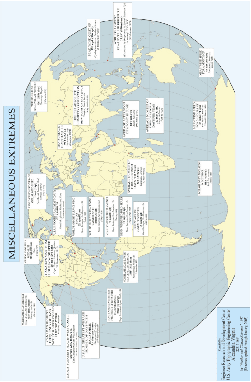
Figure description:
MISCELLANEOUS EXTREMES
MISCELLANEOUS EXTREMES
Annotations
- Red dots indicate specific locations of the recorded weather extremes. (point_marker - position: Various locations across the world map)
| Category | Record Detail | Value | Location | Date / Period |
|---|---|---|---|---|
| Sea-Level Air Pressure | North America's Highest | 31.85" (1067.7 mbars) | Northway, Alaska, USA | 31 January 1989 |
| Thunderstorms | Canada's Highest Frequency of Days | 34 per year average | Windsor, Ontario | null |
| Fog | U.S.A.'s Foggiest Place (West Coast) | Average 2,552 HRS./YR. | Cape Disappointment, Washington | 10-Year Period or More |
| Hailstorms | U.S.A.'s Greatest Average Number of Days | 9.4 days per season | Cheyenne, Wyoming | 40-Year Period |
| Wind | Greenland's Peak Wind Gust | 207 mph (333 kph) | Greenland | 8 March 1972 |
| Wind | Canada's Maximum Hourly Wind Speed | 125 mph (201 kph) | Cape Hopes Advance, Quebec | 18 November 1931 |
| Thunderstorms | North America's Highest Frequency of Days | 100 per year average | Tampa International Airport, Florida, USA | null |
| Wind | Canada's Highest Average Annual Wind Speed | 22 mph (35 kph) | Cape Warwick, Resolution Island, Northwest Territories | 1962 to 1973 |
| Fog | U.S.A.'s Foggiest Place (East Coast) | AVG. 1,580 HRS./YR. | Moose Peak Lighthouse, Mistake Island, Maine | 10-year period or more |
| Wind | World's Highest Surface Wind Peak Gust | 231 mph (372 kph) | Mount Washington, New Hampshire, USA | 12 April 1934 |
| Wind | World's Highest Surface Wind 5-Minute Speed | 188 mph (303 kph) | Mount Washington, New Hampshire, USA | 12 April 1934 |
| Wind | Mean Wind Speed for a Month | 70 mph (113 kph) | Mount Washington, New Hampshire, USA | February 1939 |
| Wind | Mean Wind Speed for 24 Hours | 128 mph (206 kph) | Mount Washington, New Hampshire, USA | 11 and 12 April 1934 |
| Wind | Highest Average Annual Wind Speed | 35 mph (56 kph) | Mount Washington, New Hampshire, USA | 1934 to 1983 |
| Sea-Level Air Pressure | North America's Lowest | 26.35" (892.3 mbars) | Matecumbe Key, Florida, USA | 2 September 1935 |
| Temperature | Sea-Surface Temperature | 96°F (35.6°C) | The Persian Gulf | 5 August 1924 |
| Humidity | Highest Absolute Humidity Observation | Dew Point of 93.2°F (34°C) | Sharjah, Saudi Arabia | July 1949-1953 |
| Dewpoint | Average Afternoon Dewpoint in June | 84°F (28.9°C) | Assab, Ethiopia | null |
| Sea-Level Air Pressure | World's Highest | 32.11" (1086.8 mbars) | Tosontsengel, Mongolia | 19 December 2001 |
| Thunderstorms | Average Number of Thunderstorm Days per Year | 242 DAYS/YR. | Kampala, Uganda | 10 Year Period |
| Thunderstorms | Average Number of Thunderstorm Days per Year | 322 DAYS/YR. | Bogor, Indonesia | 1916 to 1920 |
| Wind | Peak Wind Gust | 190 mph (306 kph) | Miyakojima Island, Ryukyu Islands | 5 September 1966 |
| Sea-Level Air Pressure | World's Lowest | 25.69" (870 mbars) | 17°N 138°E (Estimated by Dropsonde in Eye of Typhoon Tip) | 12 October 1979 |
| Wind | Mean Wind Speed for 24 Hours | 108 mph (174 kph) | Port Martin, Antarctica | 21 and 22 March 1951 |
| Wind | Mean Wind Speed for a Month | 65 mph (105 kph) | Port Martin, Antarctica | March 1951 |
| Insolation | Average Daily Insolation in December | 955 ly (463 W/m²) | South Pole, Antarctica | 1950 to 1966 |
Source: Engineer Research and Development Center, U.S. Army Topographic Engineering Center, Alexandria, Virginia Notes: The map provides various record-breaking meteorological data points including wind speed, barometric pressure, humidity, and thunderstorm frequency across different continents. Compilation date: 1997, with extremes updated through January 2003.
MIL-STD-810H PART THREE ANNEX B
PART THREE ANNEX B - Terminology
2.1 General
The documents listed in paragraph 6.1 are specified in paragraphs 3, 4, or 5 of this Method. This paragraph does not include documents cited in other paragraphs of this Method, or recommended for additional information, or as examples. While every effort has been made to ensure the completeness of this list, document users are cautioned that they must meet all specified requirements of documents cited in paragraphs 3, 4, or 5 of this Method, whether or not they are listed.
528.1-2.1 Determining and Displaying Transmissibility
Present transmissibility information using the output responses and prescribed inputs. Use the transmissibility magnitudes for both exploratory and variable frequency tests for response prominence determinations.
528.1-2.1 Hot climatic design type (A1 and B3)
The areas where hot conditions apply include most of the low latitude deserts of the world. During summer in these areas, temperatures above 43°C (110°F) occur frequently, but except for a few specific localities, temperatures will seldom be above 49°C (120°F). In winter, temperatures are not likely to be extremely low so that the low temperatures of the basic climatic design type apply. If materiel is designed only for the hot type, a special recommendation for low temperature design values should be sought. Limited portions of this area are sometimes subject to very high absolute humidity, although the highest temperatures and highest dewpoints do not occur at the same time.
The world's highest air temperatures occur in the areas identified with the hot climatic design type in Figure 1. This area is hotter than the basic design type with a 1-percent temperature of 49°C (120°F) in the hottest parts. These are primarily low latitude deserts that, in addition to very high air temperatures, concurrently experience very low relative humidity (except in the hot humid areas) and intense solar radiation. Two daily cycles, described in paragraphs 4.1.1.1 and 4.1.3.1 make up the hot design type. They are:
- a. Al Hot-dry (paragraph. (Paragraph 4.1.1.1)
b. B3 Hot-humid. (Paragraph 4.1.3.1)
2.1.1 Transmissibility Magnitudes
Develop transmissibility magnitudes by dividing the measured output amplitudes by the input amplitudes using consistent units (e.g., acceleration in gs or inches/sec²).
2.1.2 Transmissibility and Frequency
Present transmissibility information in linear-linear format. Plots or tabulations are acceptable. Present both the transmissibility and frequency information in linear units (i.e., do not use logarithms or dB of either frequency or transmissibility to compute or display the data used for response prominence determinations).
2.2 Definitions
- a. Acceptance authority. As used in this Standard, the term “acceptance authority” means the government activity (or its designated representative) having approval authority to determine vendor compliance with the requirements of this Method.
- b. Amplitude, single. See amplitude, vibratory displacement.
- c. Amplitude, vibratory displacement. Vibratory displacement amplitude is the maximum displacement of simple linear harmonic motion from the position of rest. This is also referred to as single amplitude or peak amplitude and is the maximum positive value during a given interval. It is expressed in inches, mils (0.001 inch), or mm (0.001 meter).
- d. Balancing. Balancing is a procedure by which the radial mass distribution of a rotor is adjusted so that the mass centerline approaches the geometric centerline of the rotor, and, if necessary, adjusted in order to ensure
MIL-STD-810H
METHOD 528.1
that the vibration of the journals or forces on the bearings, at a frequency corresponding to operational speed, are within specified limits.
- e. Balancing, multi-plane. Multi-plane balancing refers to any balancing procedure that requires unbalance correction in more than two axially separated correction planes.
- f. Balancing, single-plane (static). Single-plane (static) balancing is a procedure by which the mass distribution of a rigid rotor is adjusted in order to ensure the residual static unbalance is within specified limits, and that requires correction in only one plane. (Note: Single-plane balancing can be done on a pair of knife edges without rotation of the rotor, but is now more usually done on centrifugal balancing machines.)
- g. Balancing, two-plane (dynamic). Two-plane (dynamic) balancing is a procedure by which the mass distribution of a rigid rotor is adjusted in order to ensure that the residual unbalance in two specified planes is within specified limits.
- h. Critical speed. Critical speed is the speed of a rotating system that corresponds to a natural frequency of the system.
- i. Environmental vibration. Environmental vibration is vibratory force that is imposed on equipment installed aboard ships under all external conditions. The hydrodynamic force from the propeller blades interacting with the hull is usually the principal exciting force.
- j. Equipment. Equipment is any rotating or non-rotating machine that is intended to be installed aboard ship.
- k. Grade, balance quality. Balance quality grade, G, refers to the amount of permissible unbalance of a rotor. The balance quality grade is the product of the maximum permissible eccentricity (distance between the shaft axis and the rotor center of gravity (in mm)) and the rotational velocity (radians/sec). The units for balance quality grade, G, are mm/sec. By this definition, a particular grade rotor will be allowed a mass eccentricity (e=G/ω), that is inversely proportional to the operating speed.
- Internally excited vibration. Internally excited vibration is vibration of machinery generated by mass unbalance of a rotor.
- m. Isolation mount. An isolation mount is a device used to attenuate the force transmitted from the equipment to its foundation in a frequency range.
- n. Mass unbalance. Mass unbalance occurs when the mass centerline does not coincide with the geometric centerline of a rotor.
- o. Maximum design rpm. Maximum design rpm is the highest shaft rpm for which the ship is designed.
- p. Method of correction. A method of correction is a procedure, whereby the mass distribution of a rotor is adjusted to reduce unbalance or vibration due to unbalance, to an acceptable value. Corrections are usually made by adding materiel to, or removing it from, the rotor.
- q. Mode. Natural Mode is the manner or pattern of vibration at a natural frequency, and is described by its natural frequency and relative amplitude curve.
- r. Plane, correction. A correction plane is a plane transverse to the shaft axis of a rotor in which correction for unbalance is made.
- s. Plane, measuring. A measuring plane is a plane transverse to the shaft axis in which the amount and angle of unbalance is determined.
- t. Residual unbalance. Residual unbalance is unbalance of any kind that remains after balancing.
- u. Resonance. Resonance is the structural response that occurs when a linear lightly damped system is driven with a sinusoidal input at its natural frequency in which the response prominence is greater than one.
- v. Response prominence. Response prominence is a general term denoting a resonance or other distinct maximum, regardless of magnitude, in a transmissibility function, including local maxima that may exist at the frequency endpoints of the transmissibility function. Typically, a response prominence is identified by the frequency of its maximum response that is the response prominence frequency. A response prominence of a system in forced oscillation exists when any change, for both plus and minus increments however small,
in the frequency of excitation results in a decrease of the system response at the observing sensor registering the maximum. A response prominence may occur in an internal part of the equipment, with little or no outward manifestation at the vibration measurement point, and in some cases, the response may be detected by observing some other type of output function of the equipment, such as voltage, current, or any other measurable physical parameter. Instruction on how to identify response prominences is provided in Annex A.
- w. Rotor, flexible. A flexible rotor is one that does not meet the criteria for a rigid rotor and operates above its first resonance. The unbalance of a flexible rotor changes with speed. Any value of unbalance assigned to a flexible rotor must be at a particular speed. The balancing of flexible rotors requires correction in more than two planes. A rotor that operates above resonances requires balance planes of correction. A rotor that operates between the second and third resonances, for example, requires balance planes of correction.
- x. Rotor, rigid. A rotor is considered to be rigid when its unbalance can be corrected in any two arbitrarily selected planes and it operates below its first resonance. After correction, its residual unbalance does not exceed the allowed tolerance, relative to the shaft axis, at any speed up to the maximum service speed and when running under conditions that approximate closely to those of the final supporting system.
- y. Simple harmonic motion. A simple harmonic motion is a motion such that the displacement is a sinusoidal function of time.
- z. Test fixture resonance. A test fixture resonance is any enhancement of the response of the test fixture to a periodic driving force when the driving frequency is equal to a natural frequency of the test fixture.
- aa. Transmissibility. Transmissibility is the non-dimensional ratio of the response amplitude in steady-state forced vibration to the excitation amplitude. The ratio may be one of forces, displacements, velocities, or accelerations. Transmissibility is displayed in a linear-linear plot of transmissibility as a function of frequency, or in tabular form. Instructions for determining and displaying transmissibility are given in paragraph 2.1 of Annex A.
- bb. Vibration resistance. It is measured by mechanical impedance – how hard it is to make mechanical systems vibrate. It is a ratio of the exciting force to the velocity response. Low impedance implies low force and/or high velocity—a system that is easy to excite.
528.1-2.2 Identifying Response Prominences
Regardless of whether or not the transmissibility exceeds 1.0, find all local maxima in the transmissibility magnitude-frequency data and include the frequency endpoints in the list of maxima.
- a. For each of these maxima, determine if there is reason to believe that the maximum is attributable to an instrumentation error, a fixture resonance or from a numerical error related to computation of the transmissibility (round-off errors may appear as maxima). Any maxima that are attributable to an instrumentation error, fixture resonance, or numerical errors must be discarded as a potential response prominence. Fixture resonances are not permitted, and refixturing must be employed to eliminate such resonances.
- b. Examine the end points for indications that a resonance may exist outside the test frequency range.
- c. An initial decrease in transmissibility with increasing frequency above the frequency of the lower end point suggests a potential response prominence outside the lower bound of the test frequency range. If this condition is observed and is not attributed to shaker problems at low frequencies, include the lower endpoint in the candidate list of endurance test frequencies noting whether or not it affects functional or structural integrity. If this condition is not observed, the lower bound test frequency may be discarded as a potential response prominence. At these low frequencies, noticeable displacement magnitude amplifications may occur if a true response prominence exists below the lower frequency bound of testing and this fact may be used to help determine the nearby presence of a true response prominence.
- d. Similarly, an increase in transmissibility with increasing frequency near the upper bound test frequency suggests a potential response prominence outside the upper bound of the test frequency range. If this condition is observed, include the upper endpoint in the candidate list of endurance test frequencies noting whether or not it affects functional or structural integrity. If it is not observed, this frequency cannot be excluded from the list of endurance test frequencies unless other response prominence frequencies are found.
- e. Observe whether or not equipment function (if permitted by the ordering data) or structural integrity is affected at any of the frequencies used in exploratory or variable frequency testing. Include those frequencies at which equipment functional or structural integrity is affected in the candidate list of endurance test frequencies. Also include frequencies at which maxima occur in the candidate list of endurance test frequencies if the impact on functional/structural performance cannot be established.
MIL-STD-810H
METHOD 528.1 ANNEX A
- f. Examine the remaining maxima for classic signs of resonance (i.e., a moderate to rapid increase in transmissibility to the peak followed by a moderate to rapid decrease in the transmissibility with increasing frequency after the peak suggests that a response prominence may exist in this region) and include any maxima that exhibit these characteristics in the candidate list of endurance test frequencies.
528.1-2.2 Basic climatic design type
The area this type applies to includes the most densely populated and heavily industrialized parts of the world as well as the humid tropics. The entire range of basic design conditions does not necessarily apply to any one place. Each single design condition (high temperature, low temperature, and high humidity) applies to a widespread area. When taken together, the design values should provide for satisfactory materiel throughout the area involved. Tropical areas are included in the basic climatic design type because the temperature of the humid tropics is quite moderate, and the humidity is also experienced in the midlatitudes. The unique feature of the tropics that makes it important to materiel is the persistence of high humidity over long periods of time. This condition not only promotes corrosion but is an excellent environment for insect and microbiological damage.
The Basic is by far the largest of the four climatic design types. However, this large area has one constant characteristic: it has no extremely hot or cold conditions. Nevertheless, non-temperature dependent design problems within the Basic Design Type can vary with the magnitude and persistence of humidity conditions. The basic area has 1-percent cold and hot temperatures of -31.7°C (-25°F) and 43.3°C (110°F) during the worst month in the coldest and hottest parts of the regional type, respectively. The Humid Tropics are largely confined to areas between the Tropics of Capricorn and Cancer, whereas other areas of the Basic Design Type (Basic Hot & Basic Cold) range from the Tropics to the polar regions. These other areas include most of the densely populated, industrialized, and agriculturally productive land of the world.
The humid tropics and the midlatitudes (basic design type) are characterized by temperatures more moderate than the extremes of the other design types. Areas where the basic type applies are more widespread than the hot and cold design types combined. They also include most of the densely populated, highly industrialized sectors of the world. Because microbial deterioration is a function of temperature and humidity and is an inseparable condition of hot humid tropics and the mid-latitudes, consider microbial deterioration in the design of all standard general-purpose materiel. Four daily cycles, described as shown below are recognized for the basic design types. They are:
- a. (B1) Constant high humidity (paragraph 4.2.3).
- b. (B2) Variable high humidity (paragraph 4.2.4).
- c. (A2) Basic hot (paragraph 4.2.5)
- d. (C1) Basic cold (paragraph 4.2.6)
MIL-STD-810H
PART THREE
2.3 Selecting Endurance Test Frequencies
528.1-2.3 Cold and severe cold design types
The areas designated as cold, and severe cold, primarily northern North America, Greenland, northern Asia, and the Tibetan Highlands of China, were delimited because of the occurrence of low temperatures. In the area of the cold design type, temperature during the coldest month in a normal year may be colder than the basic cold extreme of -32°C (-25°F). In the severe cold areas, temperature during the coldest month in a normal year may be colder than the cold extreme of -46°C (-50°F), but colder than -51°C (-60°F) no more than 20 percent of the hours in the coldest month in the coldest part of the area (such as northern Siberia where absolute minimum temperatures as low as -68°C (-90°F) have been recorded). Because the extreme low temperatures are not controlled by a daily solar cycle, they persist for a long enough period of time for materiel to reach equilibrium at a temperature near the minimum.
The cold climatic design type areas in Figure 1 that are confined to the Northern Hemisphere have temperatures much lower than the basic cold areas, but not as low as the severe cold areas. It has a 1 percent temperature of
-45.6°C (-50°F) in the coldest parts. The cold cycle is described in paragraphs 4.2.6 - 4.3.2.
The severe cold climatic design type areas in Figure 1 have the lowest temperatures on the surface of the earth, except for Antarctica (that is not considered in this document). It has a 20-percent temperature of -51°C (-60°F) in the coldest parts. These low temperatures are found in the northern continental interiors and the Arctic. The severe cold condition is described in paragraph 4.3.3.
2.3.1 Non-responsive Prominence Frequencies Where Functional or Structural Integrity Is Affected
Include in the list of endurance test frequencies, any frequency at which a structural, functional, mechanical, or electrical anomaly has occurred (if permitted by the acceptance criteria (see paragraph 5.1.1 at the beginning of this Method, as well as Annex B, paragraph 2f(1)). Examples of these manifestations could be unexpected switch closures, unexpected changes in pressure or flow, variations in voltage, current, etc. The frequencies where any minor impairment of function occurs that does not warrant interruption of testing to develop a fix must also be included in the list of endurance test frequencies.
2.3.2 Frequencies Where Response Prominences Have Been Identified
Components may contain many parts and subassemblies that can resonate. Some components may have nonlinear characteristics such as clearances between parts or equipment mounted on isolation mounts. Therefore, the amplitude of excitation may be important relative to identifying response prominences for these components. Input amplitude dependent response prominences may potentially be the same overall resonance rather than different ones. In light of this potential, unusual test results, such as uncovering response prominences during variable frequency testing that were not uncovered during exploratory testing, need to be thoroughly investigated to not only try and determine the cause of the response prominence but to ascertain whether the response prominence is unique or part of another response prominence. Criteria for selecting response prominences for endurance testing are as follows:
- a. A transmissibility greater than 1.5 at any measurement location is sufficient to classify a maximum as a response prominence, and include the corresponding frequency in the list of endurance test frequencies. However, the converse is not necessarily true, i.e., a response prominence whose transmissibility is less than 1.5 cannot be excluded solely on the magnitude of the transmissibility. Possible explanations as to why transmissibility maxima of magnitudes less than 1.5 may still represent real response prominences are:
- (1) The transducer may not be at the point of maximum response. If probing or some other means cannot be employed to locate the point of maximum response (e.g., due to inaccessibility), then all maxima displaying the classic characteristics of a resonance that cannot be attributed to instrumentation or numerical error must be identified as response prominences, and their frequencies included in the list of endurance test frequencies.
- (2) The transducer may be at or near a response node point (location of minimal or low response in a vibration mode) at that frequency. The location of node points (as well as the locations of maximum response) can change location as changes in the drive frequency excite different modes of vibration.
- (3) The mass of the part and the amplitude of vibration of the mass that is in maximum response are not large enough to generate the forces necessary to cause structural responses of large enough magnitude at the location of the transducer.
- (4) The driving frequency is not exactly at the resonant frequency, thus the peak response is not obtained.
- b. Without further investigation, the existence of a response prominence for the remaining maxima cannot be confirmed, nor the possibility of the existence of a response prominence excluded. If practical, an attempt should be made to obtain further information to resolve this issue by probing for the maximum response location with movable transducers, listening, visually locating or feeling for the maximum response points.
- c. If it can be shown that response prominences uncovered do not compromise equipment structural/functional integrity, these response prominences do not have to be included in the endurance test. Justification should be provided in the test report as to why these response prominences have been excluded from endurance testing.
MIL-STD-810H METHOD
2.4 Guidance for Specifiers
Carefully determine all functions of the equipment that must be preserved under normal shipboard vibration. Determine the functional requirements that must be met during the vibration tests including the appropriate test acceptance criteria and include them in the procurement documents. A careful and thorough evaluation of the functional requirements will significantly reduce the potential for problems, define the basis for instrumentation selection and placement, and help in the interpretation of test results.
If possible, determine how and where to instrument the test item based on the functional requirements and expected responses, or consider requiring the vendor to make this determination. If an area of concern cannot be directly instrumented, consider instrumenting to find alternate manifestations of this area of concern (e.g., voltage fluctuations, pressure variations, noise, and contact closures). While analyses of the test and test equipment (if performed) can provide insights into possible test responses of some equipment, often neither extensive nor complicated analyses are needed, and common sense alone can often be used to establish reasonable locations of instrumentation if the functional requirements are well known. If the test vendor will determine the instrumentation scheme, depending on the equipment, consider requesting the instrumentation scheme for information or approval.
Depending on the equipment, consider requiring prior approval of frequencies used for endurance testing.
Downloaded from https://www.everyspec.com
MIL-STD-810H
METHOD 528.1 ANNEX A
(This page is intentionally blank.)
MIL-STD-810H
METHOD 528.1 ANNEX B
METHOD 528.1, ANNEX B NOTES AND ENGINEERING GUIDANCE
(This Annex contains information of a general or explanatory nature that may be helpful, but is not mandatory.)
528.1-2.4 Absolute maximum and minimum temperatures
- Absolute maximum and minimum temperatures. Figures 2 and 3 are included to show the absolute maximum and minimum temperatures that have been observed. The maps are generalized because of data limitations, and the uneven occurrence of extremes.
MIL-STD-810H PART THREE
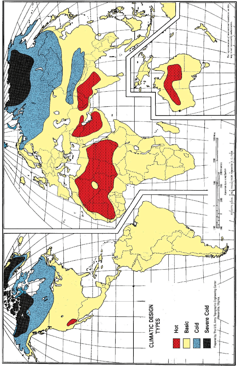
Figure description:
Key Information:
- Subject: Global map of Climatic Design Types.
- Climatic Categories:
- Hot (Red: Northern/Central Africa, Middle East, South Asia, Central Australia, and Southwest US/Mexico border.
- Basic (Yellow: Predominant category covering most of South America, Europe, sub-Saharan Africa, and Central/Southeast Asia.
- Cold (Blue: Northern North America (Canada/Alaska and Northern Eurasia (Russia.
- Severe Cold (Black: High Arctic regions including Northern Canada, Greenland, and parts of Northern Siberia.
- Source: Prepared by The U.S. Army Topographic Engineering Center, Alexandria, Virginia.
- Projection: Aitoff's Equal Area Projection adapted by V. C. Finch.
- Document Context: MIL-STD-810H, Part Three.
MIL-STD-810H
PART THREE
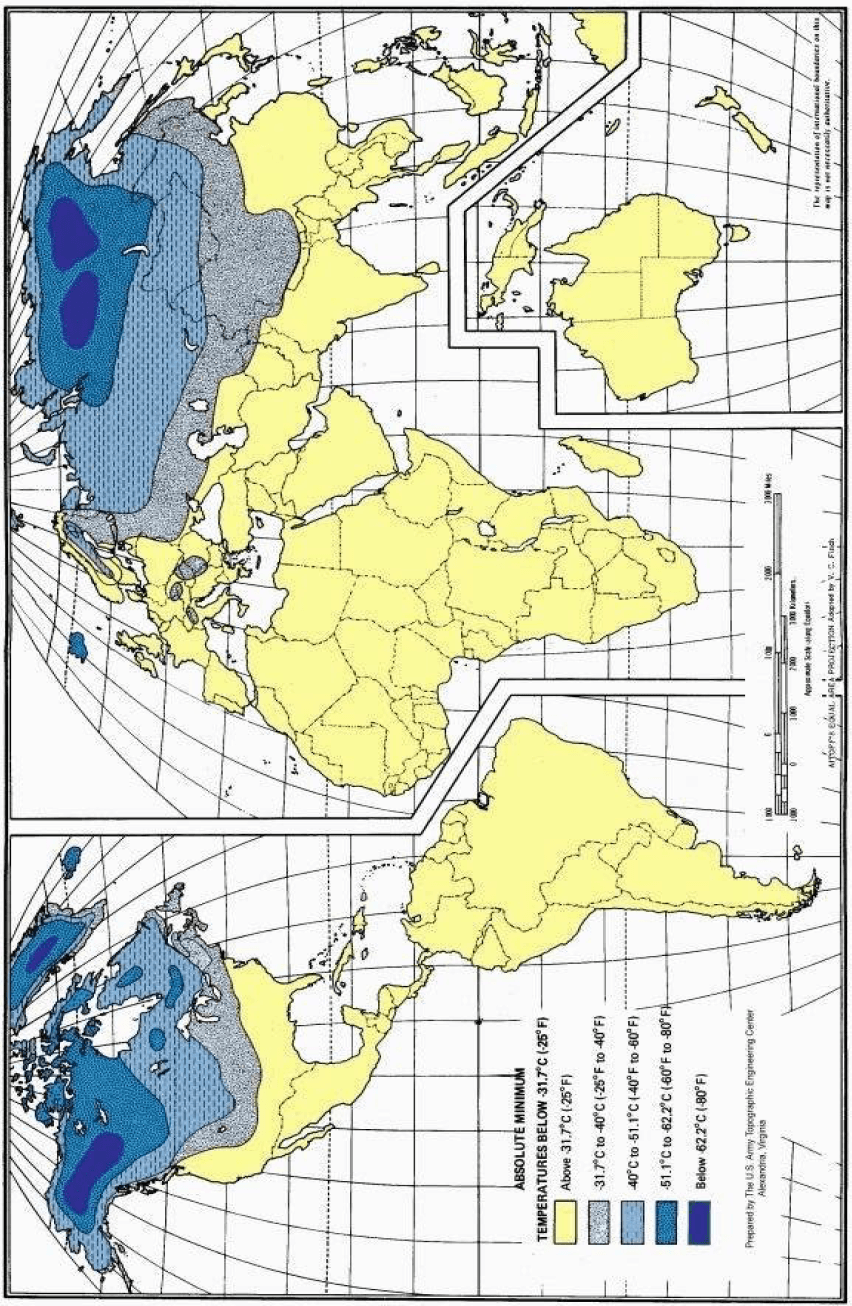
Figure description:
| Absolute Minimum Temperature Range (Celsius) | Absolute Minimum Temperature Range (Fahrenheit) | Map Color/Pattern |
|---|---|---|
| Above -31.7°C | Above -25°F | Yellow |
| -31.7°C to -40°C | -25°F to -40°F | Light Grey (Patterned) |
| -40°C to -51.1°C | -40°F to -60°F | Light Blue |
| -51.1°C to -62.2°C | -60°F to -80°F | Medium Blue |
| Below -62.2°C | Below -80°F | Dark Blue |
Key Information:
- Subject: Global distribution of absolute minimum temperatures.
- Source: U.S. Army Topographic Engineering Center; part of MIL-STD-810H Part Three.
- Key Entities: Displays extreme cold zones across the Northern Hemisphere, specifically concentrated in Northern Canada, Greenland, and Siberia (Russia.
- Projection: Aitoff's Equal Area Projection.
PART THREE-6
MIL-STD-810H PART THREE
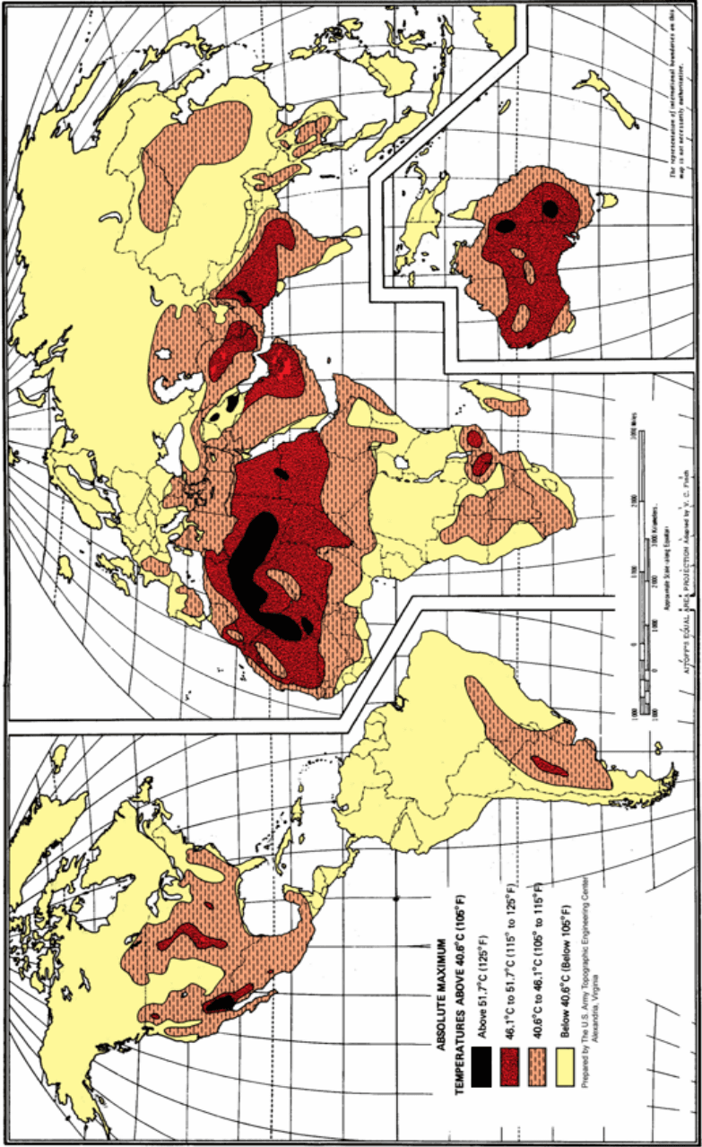
Figure description:
World Absolute Maximum Temperatures
ABSOLUTE MAXIMUM TEMPERATURES ABOVE 40.6°C (105°F
Legend
- Above 51.7°C (125°F — color: Black; symbol: Solid rectangle
- 46.1°C to 51.7°C (115° to 125°F — color: Dark Red; symbol: Solid rectangle
- 40.6°C to 46.1°C (105° to 115°F — color: Orange; symbol: Rectangle with diagonal hatching
- Below 40.6°C (Below 105°F — color: Yellow; symbol: Solid rectangle
Annotations
- Approximate Scale along Equator: 0-3000 Kilometers / 0-2000 Miles (scale_bar - position: Bottom right, above projection note)
- AITOFF'S EQUAL AREA PROJECTION Adapted by V. C. Finch (text_label - position: Bottom right corner)
- The representation of international boundaries on this map is not necessarily authoritative. (text_label - position: Vertical text on the bottom right edge)
| Temperature Range (Celsius) | Temperature Range (Fahrenheit) | Mapping Symbol/Color | Representative Geographical Regions |
|---|---|---|---|
| Above 51.7°C | Above 125°F | Solid Black | Sahara Desert (North Africa, parts of Arabian Peninsula, interior Western Australia, small pockets in Southwestern USA/Northern Mexico.) |
| 46.1°C to 51.7°C | 115° to 125°F | Solid Dark Red | Large regions of Northern and Western Africa, most of the Arabian Peninsula, Middle East (Iraq, Iran, South Asia (Pakistan, NW India, interior Australia, Gran Chaco region in South America, and Southwestern USA/Mexico border areas.)) |
| 40.6°C to 46.1°C | 105° to 115°F | Orange with Diagonal Hatching | Broad regions surrounding hotter zones in Africa, the Middle East, Southern Eurasia, Central Asia, portions of China, most of the Australian continent, Central South America, and a large portion of the Southern and Central USA. |
| Below 40.6°C | Below 105°F | Solid Yellow | Northern North America (Canada, Alaska, Northern US, Northern Eurasia, mountainous regions, equatorial rainforests, Southern South America, and most coastal/high-latitude areas.) |
Source: Prepared by The U.S. Army Topographic Engineering Center, Alexandria, Virginia Notes: The map uses Aitoff's Equal Area Projection. Data covers global landmasses with focused detail on heat-extreme regions.
PART THREE-7
MIL-STD-810H
PART THREE