|
Figure 525.2A-15 displays the stationary vibration time traces to be processed for replication error assessment. Note the time traces is nominal, and that r and c could follow a product model formulation as above because of the comparatively small envelope variation in time.
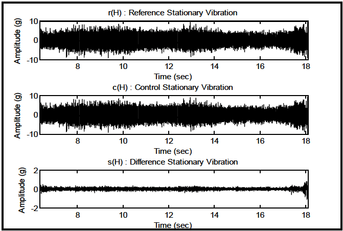
Figure description:
Stationary Vibration Analysis
r(H : Reference Stationary Vibration
| Time (sec) | Amplitude Lower Bound (g) | Amplitude Upper Bound (g) |
|---|---|---|
| 6.5 | -5.5 | 6.2 |
| 7.0 | -6.8 | 6.5 |
| 7.5 | -8.5 | 8.0 |
| 8.0 | -8.0 | 9.2 |
| 8.5 | -7.5 | 8.5 |
| 9.0 | -8.2 | 9.0 |
| 9.5 | -7.2 | 7.8 |
| 10.0 | -8.5 | 9.2 |
| 10.5 | -7.5 | 7.5 |
| 11.0 | -6.8 | 8.0 |
| 11.5 | -6.5 | 7.2 |
| 12.0 | -6.2 | 6.8 |
| 12.5 | -7.0 | 8.0 |
| 13.0 | -8.5 | 9.5 |
| 13.5 | -7.0 | 7.5 |
| 14.0 | -5.8 | 6.5 |
| 14.5 | -5.2 | 5.8 |
| 15.0 | -5.5 | 6.0 |
| 15.5 | -5.0 | 5.5 |
| 16.0 | -5.5 | 6.0 |
| 16.5 | -6.2 | 7.0 |
| 17.0 | -6.8 | 7.5 |
| 17.5 | -8.0 | 8.5 |
| 18.0 | -10.0 | 9.5 |
c(H : Control Stationary Vibration
| Time (sec) | Amplitude Lower Bound (g) | Amplitude Upper Bound (g) |
|---|---|---|
| 6.5 | -5.8 | 6.0 |
| 7.0 | -6.5 | 6.8 |
| 7.5 | -8.2 | 8.5 |
| 8.0 | -8.5 | 9.0 |
| 8.5 | -7.8 | 8.2 |
| 9.0 | -8.5 | 8.8 |
| 9.5 | -7.5 | 7.5 |
| 10.0 | -8.2 | 9.0 |
| 10.5 | -7.0 | 7.2 |
| 11.0 | -6.5 | 8.2 |
| 11.5 | -6.8 | 7.0 |
| 12.0 | -6.0 | 6.5 |
| 12.5 | -7.2 | 8.2 |
| 13.0 | -8.2 | 9.2 |
| 13.5 | -7.2 | 7.2 |
| 14.0 | -6.0 | 6.2 |
| 14.5 | -5.5 | 5.5 |
| 15.0 | -5.8 | 5.8 |
| 15.5 | -5.2 | 5.2 |
| 16.0 | -5.2 | 5.8 |
| 16.5 | -6.0 | 7.2 |
| 17.0 | -6.5 | 7.8 |
| 17.5 | -8.5 | 8.2 |
| 18.0 | -9.5 | 10.0 |
s(H : Difference Stationary Vibration
| Time (sec) | Amplitude Lower Bound (g) | Amplitude Upper Bound (g) |
|---|---|---|
| 6.5 | -0.4 | 0.5 |
| 7.0 | -0.3 | 0.4 |
| 7.5 | -0.3 | 0.3 |
| 8.0 | -0.2 | 0.3 |
| 8.5 | -0.3 | 0.3 |
| 9.0 | -0.2 | 0.2 |
| 9.5 | -0.2 | 0.3 |
| 10.0 | -0.3 | 0.3 |
| 10.5 | -0.2 | 0.2 |
| 11.0 | -0.2 | 0.3 |
| 11.5 | -0.2 | 0.2 |
| 12.0 | -0.2 | 0.2 |
| 12.5 | -0.3 | 0.3 |
| 13.0 | -0.4 | 0.4 |
| 13.5 | -0.2 | 0.3 |
| 14.0 | -0.2 | 0.2 |
| 14.5 | -0.2 | 0.3 |
| 15.0 | -0.2 | 0.2 |
| 15.5 | -0.2 | 0.3 |
| 16.0 | -0.2 | 0.2 |
| 16.5 | -0.3 | 0.3 |
| 17.0 | -0.4 | 0.5 |
| 17.5 | -0.8 | 0.8 |
| 18.0 | -1.5 | 1.0 |
Notes: The charts display three high-frequency vibration signals over time. The 'Amplitude Lower Bound' and 'Amplitude Upper Bound' columns in the data tables approximate the envelope of the signal noise observed in the graphs.
Figure 525.2A-15. Stationary vibration time traces - r, c, and s.
The replication error is assessed under the stationary random vibration assumption as follows:
- (1) Probability density estimates are generated for r and c.
- (2) s qq-plot is generated to examine the difference time trace for normality.
(3) Fraction-of-Time (FOT) distribution for s
(4) ASD estimates are determined for r, c and s.
To examine the Gaussian form of the stationary vibration trace, the composite histogram (probability density function estimate) for r and c is plotted in Figure 525.2A-16, with the tail behavior enhanced. The time trace information is long-tailed because of the presence of the time-varying mean-square amplitude. "G" represents the Gaussian histogram on the plot legend.
|
|
Figure 525.2A-17 provides a qq-plot for s for Gaussian quantiles. The tail behavior of s would seem to indicate that the peak and valley values are somewhat larger than and smaller, respectively, than a Gaussian. Even though the Gaussian portion (good fit to straight line is greater than in the transient vibration case).
MIL-STD-810H METHOD 525.2 ANNEX A
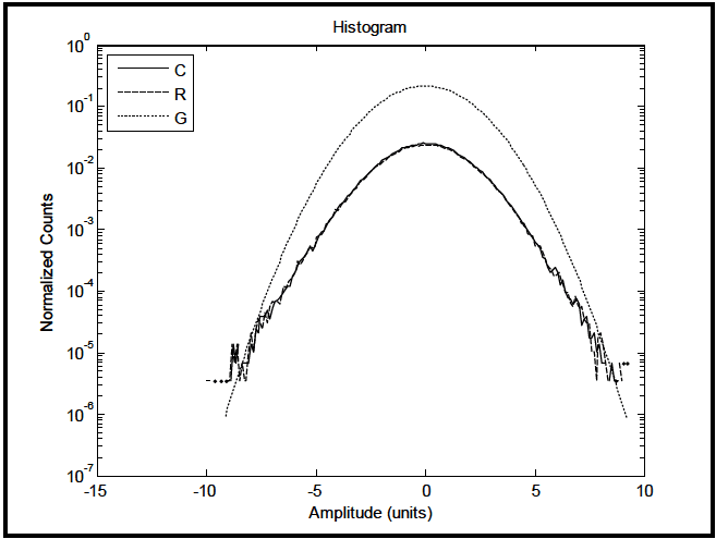
Figure description:
Histogram Figure with Logarithmic Normalized Counts
Histogram
Legend
- C — color: black; symbol: Solid line
- R — color: black; symbol: Dashed line
- G — color: black; symbol: Dotted line
| Amplitude (units) | Normalized Counts (C) | Normalized Counts (R) | Normalized Counts (G) |
|---|---|---|---|
| -10.0 | null | null | 3.5e-06 |
| -9.5 | null | null | 3.5e-06 |
| -9.0 | 1.1e-05 | 4.0e-06 | 1.0e-07 |
| -8.5 | 1.5e-05 | 1.5e-05 | 4.0e-07 |
| -8.0 | 2.0e-05 | 2.0e-05 | 1.5e-06 |
| -7.5 | 3.0e-05 | 3.5e-05 | 6.0e-06 |
| -7.0 | 5.0e-05 | 6.0e-05 | 2.5e-05 |
| -6.5 | 8.0e-05 | 1.0e-04 | 9.0e-05 |
| -6.0 | 1.2e-04 | 1.5e-04 | 2.5e-04 |
| -5.5 | 2.5e-04 | 3.5e-04 | 8.0e-04 |
| -5.0 | 8.0e-04 | 1.0e-03 | 2.0e-03 |
| -4.5 | 1.8e-03 | 2.2e-03 | 5.5e-03 |
| -4.0 | 3.0e-03 | 3.5e-03 | 1.1e-02 |
| -3.5 | 6.5e-03 | 7.0e-03 | 2.2e-02 |
| -3.0 | 1.0e-02 | 1.1e-02 | 4.5e-02 |
| -2.5 | 1.4e-02 | 1.5e-02 | 8.0e-02 |
| -2.0 | 1.8e-02 | 1.9e-02 | 1.2e-01 |
| -1.5 | 2.2e-02 | 2.3e-02 | 1.7e-01 |
| -1.0 | 2.4e-02 | 2.4e-02 | 2.0e-01 |
| -0.5 | 2.5e-02 | 2.5e-02 | 2.1e-01 |
| 0.0 | 2.5e-02 | 2.5e-02 | 2.2e-01 |
| 0.5 | 2.5e-02 | 2.5e-02 | 2.1e-01 |
| 1.0 | 2.4e-02 | 2.4e-02 | 2.0e-01 |
| 1.5 | 2.2e-02 | 2.3e-02 | 1.7e-01 |
| 2.0 | 1.8e-02 | 1.9e-02 | 1.2e-01 |
| 2.5 | 1.4e-02 | 1.5e-02 | 8.0e-02 |
| 3.0 | 1.0e-02 | 1.1e-02 | 4.5e-02 |
| 3.5 | 6.5e-03 | 7.0e-03 | 2.2e-02 |
| 4.0 | 3.0e-03 | 3.5e-03 | 1.1e-02 |
| 4.5 | 1.8e-03 | 2.2e-03 | 5.5e-03 |
| 5.0 | 8.0e-04 | 1.0e-03 | 2.0e-03 |
| 5.5 | 2.5e-04 | 3.5e-04 | 8.0e-04 |
| 6.0 | 1.2e-04 | 1.5e-04 | 2.5e-04 |
| 6.5 | 8.0e-05 | 1.0e-04 | 9.0e-05 |
| 7.0 | 5.0e-05 | 6.0e-05 | 2.5e-05 |
| 7.5 | 3.0e-05 | 3.5e-05 | 6.0e-06 |
| 8.0 | 2.0e-05 | 2.0e-05 | 1.5e-06 |
| 8.5 | 1.5e-05 | 1.5e-05 | 4.0e-07 |
| 9.0 | 4.0e-06 | 4.0e-06 | 7.0e-06 |
| 9.5 | null | null | 7.0e-06 |
|
Figure 525.2A-16. Stationary vibration probability density function estimates.
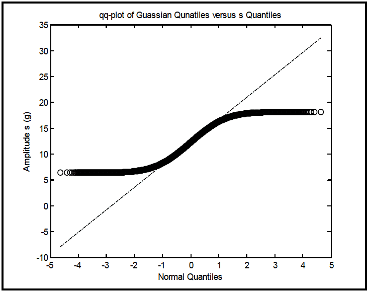
Figure description:
qq-plot of Guassian Qunatiles versus s Quantiles
qq-plot of Guassian Qunatiles versus s Quantiles
Legend
- Amplitude s (g — color: black; symbol: Open circle
- Reference Line — color: black; symbol: Dashed-dotted line
| Normal Quantiles | Amplitude s (g) | Reference Line |
|---|---|---|
| -4.6 | 6.5 | -8.4 |
| -4.2 | 6.5 | -6.6 |
| -3.8 | 6.5 | -4.8 |
| -3.4 | 6.5 | -3.0 |
| -3.0 | 6.5 | -1.2 |
| -2.6 | 6.6 | 0.6 |
| -2.2 | 6.7 | 2.4 |
| -1.8 | 7.1 | 4.2 |
| -1.4 | 7.8 | 6.0 |
| -1.0 | 8.8 | 7.8 |
| -0.6 | 10.1 | 9.6 |
| -0.2 | 11.6 | 11.4 |
| 0.0 | 12.3 | 12.3 |
| 0.2 | 13.1 | 13.2 |
| 0.6 | 14.6 | 15.0 |
| 1.0 | 15.9 | 16.8 |
| 1.4 | 17.1 | 18.6 |
| 1.8 | 17.8 | 20.4 |
| 2.2 | 18.1 | 22.2 |
| 2.6 | 18.2 | 24.0 |
| 3.0 | 18.2 | 25.8 |
| 3.4 | 18.2 | 27.6 |
| 3.8 | 18.2 | 29.4 |
| 4.2 | 18.2 | 31.2 |
| 4.6 | 18.2 | 33.0 |
Notes: Note that 'Guassian' and 'Qunatiles' are misspelled in the original image title. The reference line follows a linear trend of approximately y = 4.5x + 12.3, representing the expected distribution if it were normal.
|
Figure 525.2A-17. Stationary vibration q-q plot for s versus Gaussian.