TPP replication error assessment is most stringent for specifying tolerance criteria being that the tolerance criteria must be satisfied for the correlated time points, point-by-point. Replication error averages for STA is most easily defined for application to s, as opposed to application to r and c individually, and then seeking to compare STA r estimates with STA c estimates. Annex B discusses some complications with individual STA application. For Annex A post-test processing, using STA directly centers upon the statistical characteristics of s under short-time averaging. Figures 525.2A-26 and 525.2A-27 display short-time averaging for the mean and root-mean-square of time trace s over the entire time trace displayed in Figure 525.2A-3d-f for 0.05 and 0.20 second averaging times. An averaging time of 0.05 seconds for a bandwidth of 2000 Hz provides 5 percent normalized random error in the root-mean-square estimate, and an averaging time of 0.20 seconds for the SESA bandwidth provides a 5 percent normalized random error in the mean-square estimate. For AC coupled instrumentation measurements, the short-time average mean is near zero - not particularly meaningful, but is computed for completeness. It is clear from these figures that the rate of change of the time trace is too great in the transient vibration, and shock tails of the time trace to provide meaningful estimates by averaging in time. Thus, tolerance information in these two tails requires another basis, e.g., TPP.
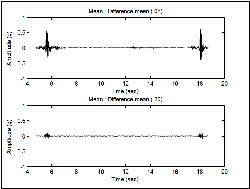
Figure description:
Mean : Difference mean (.05
| Time (sec) | Amplitude (g) |
|---|---|
| 4.6 | -0.01 |
| 4.8 | 0.03 |
| 5.0 | -0.04 |
| 5.2 | 0.02 |
| 5.4 | -0.08 |
| 5.5 | 0.26 |
| 5.6 | 0.56 |
| 5.7 | -0.51 |
| 5.8 | 0.48 |
| 5.9 | -0.22 |
| 6.0 | 0.08 |
| 6.2 | -0.05 |
| 6.4 | 0.08 |
| 8.0 | 0.02 |
| 10.0 | -0.01 |
| 12.0 | 0.03 |
| 14.0 | -0.02 |
| 16.0 | 0.01 |
| 17.2 | 0.05 |
| 17.4 | -0.12 |
| 17.6 | 0.15 |
| 17.8 | -0.42 |
| 18.0 | 0.28 |
| 18.1 | 0.63 |
| 18.2 | -0.38 |
| 18.4 | 0.18 |
| 18.6 | -0.06 |
| 18.8 | 0.04 |
Mean : Difference mean (.20
| Time (sec) | Amplitude (g) |
|---|---|
| 4.6 | 0.002 |
| 4.8 | -0.003 |
| 5.0 | 0.004 |
| 5.2 | -0.002 |
| 5.4 | 0.01 |
| 5.5 | -0.06 |
| 5.6 | 0.08 |
| 5.7 | -0.12 |
| 5.8 | 0.10 |
| 5.9 | -0.04 |
| 6.0 | 0.02 |
| 6.2 | -0.01 |
| 6.4 | 0.01 |
| 8.0 | 0.002 |
| 10.0 | -0.001 |
| 12.0 | 0.003 |
| 14.0 | -0.002 |
| 16.0 | 0.001 |
| 17.2 | 0.01 |
| 17.4 | -0.02 |
| 17.6 | 0.03 |
| 17.8 | -0.09 |
| 18.0 | 0.06 |
| 18.1 | 0.12 |
| 18.2 | -0.10 |
| 18.4 | 0.04 |
| 18.6 | -0.01 |
| 18.8 | 0.005 |
Notes: The figure contains two time-series plots showing signal amplitude over time. Both charts display a low-amplitude background signal with two prominent bursts of activity around 5-6 seconds and 17-19 seconds. The top plot (.05 shows significantly higher peak amplitudes compared to the bottom plot (.20.))
|
Figure 525.2A-26. Short-time averaging for difference mean.
MIL-STD-810H METHOD 525.2 ANNEX A
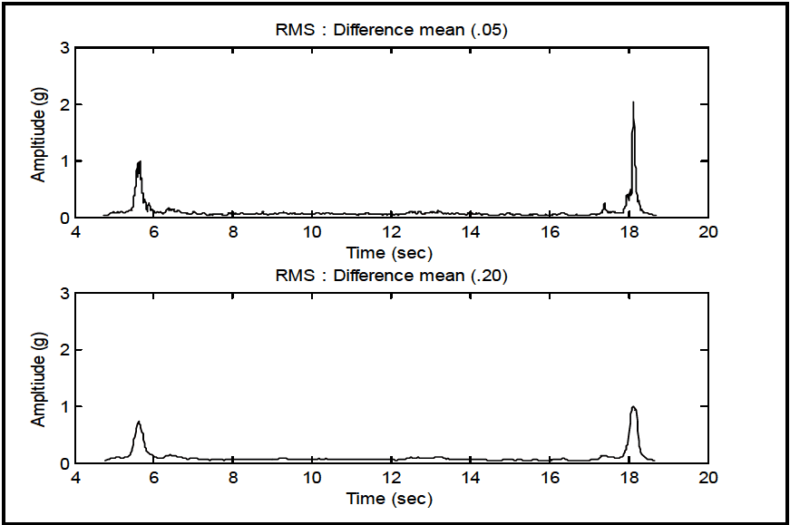
Figure description:
Amplitude Comparison of RMS Difference Mean
RMS : Difference mean (.05
| Time (sec) | Amplitude (g) |
|---|---|
| 4.7 | 0.05 |
| 5.0 | 0.12 |
| 5.3 | 0.15 |
| 5.4 | 0.40 |
| 5.5 | 0.85 |
| 5.6 | 1.00 |
| 5.7 | 0.25 |
| 5.8 | 0.35 |
| 6.0 | 0.10 |
| 6.5 | 0.18 |
| 7.0 | 0.08 |
| 8.0 | 0.09 |
| 9.0 | 0.07 |
| 10.0 | 0.08 |
| 11.0 | 0.06 |
| 12.0 | 0.08 |
| 13.0 | 0.09 |
| 14.0 | 0.06 |
| 15.0 | 0.07 |
| 16.0 | 0.06 |
| 17.0 | 0.08 |
| 17.4 | 0.28 |
| 17.8 | 0.10 |
| 17.9 | 0.45 |
| 18.1 | 2.05 |
| 18.2 | 0.45 |
| 18.4 | 0.15 |
| 18.7 | 0.05 |
RMS : Difference mean (.20
| Time (sec) | Amplitude (g) |
|---|---|
| 4.7 | 0.06 |
| 5.0 | 0.11 |
| 5.3 | 0.18 |
| 5.4 | 0.40 |
| 5.6 | 0.75 |
| 5.8 | 0.25 |
| 6.0 | 0.15 |
| 6.5 | 0.18 |
| 7.0 | 0.08 |
| 8.0 | 0.07 |
| 9.0 | 0.08 |
| 10.0 | 0.09 |
| 11.0 | 0.07 |
| 12.0 | 0.09 |
| 13.0 | 0.08 |
| 14.0 | 0.07 |
| 15.0 | 0.08 |
| 16.0 | 0.06 |
| 17.0 | 0.08 |
| 17.4 | 0.15 |
| 17.8 | 0.12 |
| 18.1 | 1.00 |
| 18.3 | 0.20 |
| 18.5 | 0.10 |
| 18.7 | 0.06 |
Notes: The figure consists of two subplots showing the RMS difference mean at two different window sizes (.05 and .20. The plots demonstrate two main impulse events at approximately 5.6 and 18.1 seconds. Smoothing is evident in the .20 plot, which shows lower peak amplitudes compared to the .05 plot.)
Figure 525.2A-27. Short-time averaging for difference root-mean-square.
Justification for using short-time average estimates for error assessment is that for stationary random processing, the principal comparison with the ASD estimate in the frequency domain is an average, and for shock processing, the principal comparison with the SRS estimate in the single-degree of freedom natural frequency domain is an integrated (or averaged) nonlinear type estimate. Annex B defines time average estimates in continuous form, and in digital form for a rudimentary description of the underlying non-stationary random process. The averaging time is arbitrary, but generally will be such that the normalized bias error is a minimum, and the normalized statistical error in the root- mean-square estimate under Gaussian assumptions is no more than 0.05. The expressions for the normalized root- mean-square error and normalized mean-square error are provided in Annex B.
This concludes Annex A and processing of selected information supplied for SESA TWR. As technology evolves, the information in this Annex will also evolve. Significant evolution needs to take place in understanding the extent of signal compensation, how it is performed, what its limitations are, and just general overall TWR control strategy understanding. This evolution will feed directly into the development of realistic tolerance limits based upon replication error assessment.
Downloaded from https://www.everyspec.com
MIL-STD-810H METHOD 525.2 ANNEX A
(This page is intentionally blank.)