Figure 525.2A-20 displays the shock time traces that will be processed for replication error assessment. Note that time trace, s, is not nominal in the area of maximum shock. The maximum/minimum values for each trace are given by r: -22.84/35.24; c(H): -24.28/39.76; and s(H): -4.11/4.78.
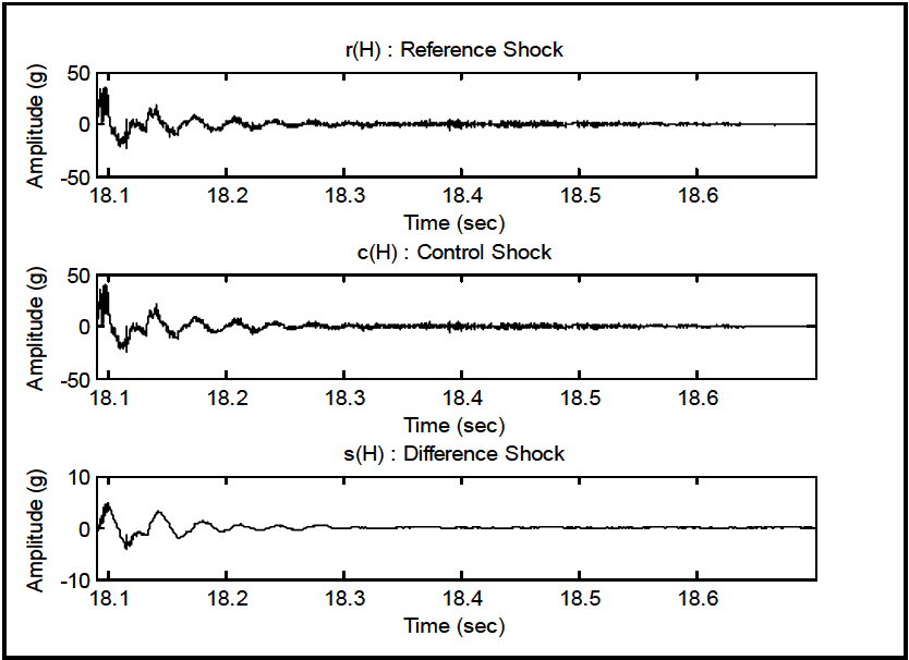
Figure description:
Shock Signal Analysis: Reference, Control, and Difference
r(H : Reference Shock
| Time (sec) | Amplitude (g) |
|---|---|
| 18.08 | 0.0 |
| 18.09 | 40.0 |
| 18.11 | -25.0 |
| 18.14 | 20.0 |
| 18.16 | -15.0 |
| 18.18 | 10.0 |
| 18.21 | -10.0 |
| 18.24 | 8.0 |
| 18.27 | -4.0 |
| 18.30 | 4.0 |
| 18.34 | -2.0 |
| 18.38 | 2.0 |
| 18.42 | -1.0 |
| 18.50 | 0.5 |
| 18.60 | 0.0 |
| 18.70 | 0.0 |
c(H : Control Shock
| Time (sec) | Amplitude (g) |
|---|---|
| 18.08 | 0.0 |
| 18.09 | 35.0 |
| 18.11 | -20.0 |
| 18.14 | 16.5 |
| 18.16 | -11.5 |
| 18.18 | 8.0 |
| 18.21 | -8.2 |
| 18.24 | 6.8 |
| 18.27 | -3.2 |
| 18.30 | 3.2 |
| 18.34 | -1.7 |
| 18.38 | 1.7 |
| 18.42 | -0.8 |
| 18.50 | 0.4 |
| 18.60 | 0.0 |
| 18.70 | 0.0 |
s(H : Difference Shock
| Time (sec) | Amplitude (g) |
|---|---|
| 18.08 | 0.0 |
| 18.09 | 5.0 |
| 18.11 | -5.0 |
| 18.14 | 3.5 |
| 18.16 | -3.5 |
| 18.18 | 2.0 |
| 18.21 | -1.8 |
| 18.24 | 1.2 |
| 18.27 | -0.8 |
| 18.30 | 0.8 |
| 18.34 | -0.3 |
| 18.38 | 0.3 |
| 18.42 | -0.2 |
| 18.50 | 0.1 |
| 18.60 | 0.0 |
| 18.70 | 0.0 |
Notes: The figure contains three subplots showing shock signals over time. The Reference Shock r(H and Control Shock c(H have an amplitude range of -50 to 50 g, while the Difference Shock s(H has a smaller range of -10 to 10 g. All signals are measured between approximately 18.08 and 18.70 seconds.)))
Figure 525.2A-20. Shock time traces - r, c, and s.
The replication error is assessed under the shock assumption as follows:
- a. An r versus c cross plot is generated.
- b. s qq-plot is generated to examine the difference time trace for normality.
- (1) Pseudo-velocity SRS assessment for r and c.
- (2) ESD estimates are determined for r, c, and s under a shock time trace assumption.
For the shock segment, a cross plot of r versus c provides useful information with regard to the positive and negative peaks. However, from the form of the r and c time traces, it is obvious that histograms and empirical q-q plots versus the Gaussian will yield little useful information. Figure 525.2A-21 provides a cross-plot of r versus c.
MIL-STD-810H METHOD 525.2 ANNEX A
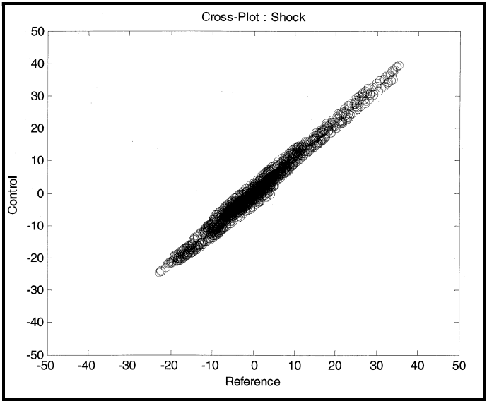
Figure description:
Cross-Plot : Shock
Cross-Plot : Shock
| Reference | Control |
|---|---|
| -23.0 | -24.5 |
| -20.0 | -21.5 |
| -15.0 | -16.0 |
| -10.0 | -11.0 |
| -5.0 | -5.5 |
| 0.0 | 0.5 |
| 5.0 | 6.5 |
| 10.0 | 12.5 |
| 15.0 | 18.0 |
| 20.0 | 24.0 |
| 25.0 | 29.5 |
| 30.0 | 35.0 |
| 35.0 | 39.5 |
Notes: The figure is a scatter plot showing a strong positive linear correlation between 'Reference' and 'Control' values. The data points form a dense, narrow cloud with a slope slightly greater than 1, centered around the origin. The points range from roughly -23 to 35 on the Reference axis and -25 to 40 on the Control axis.
Figure 525.2A-21. r versus c cross-plot.
|
Even though "s" will not display Gaussian character, some indication of its non-Gaussian character can be useful. Figure 525.2A-22 provides a q-q plot of s versus the Gaussian distribution. Clearly, the sample quantiles from "s" in the tails far exceed any Gaussian model that can be fit to s.
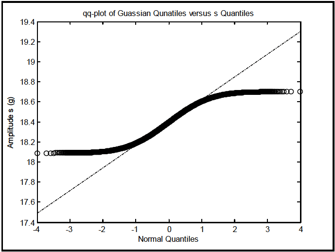
Figure description:
qq-plot of Guassian Qunatiles versus s Quantiles
qq-plot of Guassian Qunatiles versus s Quantiles
Legend
- s Quantiles — color: black; symbol: circle
- Reference Line — color: black; symbol: dashed-dotted line
| Normal Quantiles | Amplitude s (g) | Reference Line |
|---|---|---|
| -4.0 | 18.09 | 17.50 |
| -3.5 | 18.09 | 17.61 |
| -3.0 | 18.10 | 17.73 |
| -2.5 | 18.11 | 17.84 |
| -2.0 | 18.13 | 17.95 |
| -1.5 | 18.16 | 18.06 |
| -1.0 | 18.22 | 18.18 |
| -0.5 | 18.31 | 18.29 |
| 0.0 | 18.40 | 18.40 |
| 0.5 | 18.49 | 18.51 |
| 1.0 | 18.58 | 18.63 |
| 1.5 | 18.65 | 18.74 |
| 2.0 | 18.68 | 18.85 |
| 2.5 | 18.69 | 18.96 |
| 3.0 | 18.70 | 19.08 |
| 3.5 | 18.70 | 19.19 |
| 4.0 | 18.70 | 19.30 |
|
Figure 525.2A-22. Shock q-q plot for s versus Gaussian.