Specific Tolerances For All Random Vibration Tests (including the broadband component of mixed random and sinusoidal vibration tests and the fixed and swept narrowband components of mixed broadband and narrowband random vibration tests)
| Parameter | Tolerance | |
|---|---|---|
| Number (n) of independent statistical degrees of freedom (DOF) for control of the specified ASD. | n > 120 | |
| Composite Control: Maximum deviation of the composite control ASD in relation to the specified ASD.1 | ± 3 dB below 500 Hz ± 6 dB above 500 Hz ± 10% overall grms | |
| Multi-point Control: Maximum deviation of any individual control channel ASD in relation to the specified ASD.2 | Average Control ± 6 dB below 500 Hz ± 9 dB above 500 Hz | Extremal Control - 6 dB / + 3 dB below 500 Hz - 9 dB / + 6 dB above 500 Hz ± 25% overall grms |
| Cross-axis Motion: ASD measured with the same number of DOF as in the test axis, along the mutually orthogonal directions, in relation to the in-axis specified ASD. | Less than 50% below 500 Hz Less than 100% above 500 Hz Less than the relevant specified ASD for the given cross-axis. | |
| Frequency sweep rate | ± 10% of stated rate | |
| Test time duration | ± 5% of stated duration | |
| Amplitude distribution of the instantaneous values of the random vibration measured at the drive signal. | Nominally Gaussian (Refer to paragraph 2.4 for amplitude distribution discussion) | |
Composite Control is defined as: The ASD computed as either the average, maximum, or minimum (depending on control method) of all feedback channels deemed as control channels in a multi-point control scenario or the single control channel in a single-point control scenario. As discussed in paragraph 4.2.1.1 multi-point control is encouraged.
- ² If using minimum control, the negative tolerance will be that of the Composite Control.
The default assumption for all ASD references provided in this document is that the associated probability density function (pdf) is of Gaussian form. Generally, unless documentation from field data indicates otherwise, the drive-limiting option (often referred to as three-sigma clipping) should not be invoked. However, it is recognized that there are scenarios such as test equipment displacement limitations or power amplifier voltage or current limitations that could be resolved by invoking the drive limiting control parameter. When invoking the drive signal limiting feature on a Gaussian drive signal, the limiting threshold should never be set to less than three standard deviations (3-sigma). In addition, the test engineer or program engineer responsible for the test article should approve the operation and it should be properly documented within the test report.
When an ASD is being generated to serve as a reference for a vibration test, careful examination of field measured response probability density information should be performed. The probability density/distribution function should be estimated and compared with that of a theoretical Gaussian probability density/distribution. If there is strong evidence of departure from the Gaussian distribution then an accurate estimate of the higher moments – primarily kurtosis and skewness should be made, cognizant of the substantial increased amount of measurement information needed to estimate higher order moments accurately. Skewness and kurtosis are the third and fourth standardized moments about the mean computed as:
MIL-STD-810H
METHOD 514.8
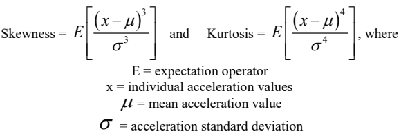
Figure description:
Mathematical Formulas and Definitions
- Skewness:
- Kurtosis:
Variables:
- E: Expectation operator
- x: Individual acceleration values
- : Mean acceleration value
- : Acceleration standard deviation
A Gaussian process has a skewness equal to 0 and a kurtosis equal to 3. Skewness is a measure of the asymmetry of the probability distribution of a random variable while kurtosis is a measure of “peakedness” or “flatness” of the distribution.
If analysis shows the data to be highly non-Gaussian, one may consider either of the following:
- (1) Employing TWR techniques (that will generally preserve the measured pdf and the distribution in time of the time history characteristics e.g., peaks and valleys, that provide for kurtosis differing from the Gaussian theoretical value).
- (2) Employing a control algorithm capable of drive signal synthesis per user defined kurtosis and “matching” the measurement pdf within some level of statistical confidence. All control systems do not necessarily assume the same model for generating non-Gaussian input and most control system software ignore the form of the pdf. Use of a control system that does not take account of the form of the pdf is discouraged unless it can be demonstrated that the pdf of the synthesized data is comparable (via statistical test) to that of the measured data upon which the test reference is based. This assumes a single measured test reference with non-Gaussian behavior. When several measured test references are present the overall non-Gaussian behavior may be due to “mixture distribution” effects, in which case an analyst must be consulted for recommendations as to a way to proceed.
In the event TWR or user defined kurtosis options as defined above are employed to address non-Gaussian scenarios, the time compression techniques outlined in Annex A paragraph 2.2 are not applicable.
The test engineer or program engineer responsible for the test article should approve any deviation from the standard Gaussian process and any deviations should be properly documented within the test report by time history plots, skewness/kurtosis estimates and probability density function estimate plots.
514.8 -III. Sinusoidal Vibration Test Tolerances
Specific Tolerances For All Sinusoidal Tests (including fixed, swept and stepped sine tests as well as the fixed and swept sinusoidal components of mixed random and sinusoidal tests)
| Parameter | Tolerance | |
|---|---|---|
| Frequency | ± 0.1 % | |
| Composite Control: Maximum deviation of the composite control1 tone level(s) in relation to the specified tone level(s). | ± 10% | |
| Multi-point Control: Maximum deviation of the individual control channel tone levels in relation to the specified tone level(s).2 | Average Control ± 25% below 500 Hz ± 50% above 500 Hz | Maxi Control +10% / -25% below 500 Hz +10% / -50% above 500Hz |
| Cross-axis Motion: Tone levels measured along the mutually orthogonal directions, in relation to the in-axis specified level(s). | Less than 50% below 500 Hz Less than 100% above 500 Hz Less than the relevant specified levels for the given cross-axis. | |
| Frequency sweep rate | ± 10% of stated rate | |
| Test time duration | ± 5% of stated duration | |
| Difference between the unfiltered signal and filtered acceleration signal3 | ± 5% on the grms values4 | |
1
- Composite Control is defined as: The Line Spectrum computed as either the average, maximum, or minimum (depending on control method) of all feedback channels deemed as control channels in a multi-point control scenario or the single control channel in a single-point control scenario. As discussed in paragraph 4.2.1.1
- 2 If using minimum control, the negative tolerance will be that of the Composite Control.
- 3 Distortion of the sinusoidal signal can occur particularly when using hydraulic actuators. If distortion of the sinusoidal signal is suspected, the unfiltered signal and filtered acceleration signal should be compared. A signal tolerance of ±5 percent corresponds to a distortion of 32 percent by utilization of the formula:
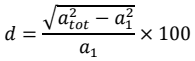
Figure description:
atot - a² d × 100 a1
where: a₁ = grms value of acceleration at the driving frequency;
atot total grms of the applied acceleration (including the value of α₁).
- 4 The grms of a sinusoid equals 0.707 times peak g. It is not related to grms of a random (g2/Hz) spectrum; do NOT use this to compare sine criteria (g) to random criteria (g2/Hz).