516.8 SHOCK CONTENTS
| Paragraph | Page | |
|---|---|---|
| 1. | SCOPE | 1 |
| 1.1 | PURPOSE | 1 |
| 1.2 | APPLICATION | 1 |
| 1.3 | LIMITATIONS | 1 |
| 2. | TAILORING GUIDANCE. | 2 |
| 2.1 | SELECTING THE SHOCK METHOD. | 2 |
| 2.1.1 | EFFECTS OF SHOCK | 2 |
| 2.1.2 | SEQUENCE AMONG OTHER METHODS | 2 |
| 2.2 | SELECTING A PROCEDURE. | 3 |
| 2.2.1 | PROCEDURE SELECTION CONSIDERATIONS | 3 |
| 2.2.2 | DIFFERENCE AMONG PROCEDURES | 4 |
| 2.3 | DETERMINE TEST LEVELS AND CONDITIONS | 5 |
| 2.3.1 | GENERAL CONSIDERATIONS - TERMINOLOGY AND PROCESSING PROCEDURES WITH ILLUSTRATION. | 5 |
| 2.3.1.1 | THE SHOCK MODEL | 5 |
| 2.3.1.2 | LABORATORY SHOCK TEST OPTIONS | 7 |
| 2.3.2 | TEST CONDITIONS | 9 |
| 2.3.2.1 | SRS BASED ON MEASURED DATA | 10 |
| 2.3.2.2 | SRS IN THE ABSENCE OF MEASURED DATA | 10 |
| 2.3.2.3 | CLASSICAL SHOCK PULSE | 12 |
| 2.3.3 | TEST AXES AND NUMBER OF SHOCK EVENTS - GENERAL CONSIDERATIONS | 16 |
| 2.3.3.1 | SPECIAL CONSIDERATIONS FOR COMPLEX TRANSIENTS | 16 |
| 2.4 | TEST ITEM CONFIGURATION | 16 |
| 3. | INFORMATION REQUIRED | 16 |
| 3.1 | PRETEST | 16 |
| 3.2 | DURING TEST | 17 |
| 3.3 | POST-TEST | 17 |
| 4. | TEST PROCESS | 17 |
| 4.1 | TEST FACILITY | 17 |
| 4.2 | CONTROLS | 18 |
| 4.2.1 | CALIBRATION. | 18 |
| 4.2.2 | TOLERANCES | 18 |
| 4.2.2.1 | CLASSICAL PULSES AND COMPLEX TRANSIENT PULSE-TIME DOMAIN | 18 |
| 4.2.2.2 | COMPLEX TRANSIENT PULSES-SRS | 18 |
| 4.3 | TEST INTERRUPTION | 19 |
| 4.3.1 | INTERRUPTION DUE TO LABORATORY EQUIPMENT MALFUNCTION | 19 |
| 4.3.2 | INTERRUPTION DUE TO TEST ITEM OPERATION FAILURE | 19 |
| 4.4 | INSTRUMENTATION | 20 |
| 4.5 | DATA ANALYSIS | 21 |
| 4.6 | TEST EXECUTION | 22 |
| 4.6.1 | PREPARATION FOR TEST. | 22 |
| 4.6.1.1 | PRELIMINARY GUIDELINES | 22 |
| 4.6.1.2 | PRETEST CHECKOUT | 22 |
| 4.6.1.3 | PROCEDURES' OVERVIEW | 22 |
MIL-STD-810H
METHOD 516.8
CONTENTS – Continued
| Paragraph | Page | |
|---|---|---|
| 4.6.2 | FUNCTIONAL SHOCK (PROCEDURE I) | 22 |
| 4.6.2.1 | TEST CONTROLS - FUNCTIONAL SHOCK (PROCEDURE I) | 24 |
| 4.6.2.2 | TEST TOLERANCES - FUNCTIONAL SHOCK (PROCEDURE I) | 24 |
| 4.6.2.3 | TEST PROCEDURE I - FUNCTIONAL SHOCK (PROCEDURE I) | 24 |
| 4.6.3 | TRANSPORTATION SHOCK (PROCEDURE II) | 25 |
| 4.6.3.1 | TEST CONTROLS - TRANSPORTATION SHOCK (PROCEDURE II) | 26 |
| 4.6.3.2 | TEST TOLERANCES - TRANSPORTATION SHOCK (PROCEDURE II) | 26 |
| 4.6.3.3 | TEST PROCEDURE - TRANSPORTATION SHOCK (PROCEDURE II) | 26 |
| 4.6.4 | FRAGILITY (PROCEDURE III) | 26 |
| 4.6.4.1 | TEST CONTROLS - FRAGILITY (PROCEDURE III) | 29 |
| 4.6.4.2 | TEST TOLERANCES - FRAGILITY (PROCEDURE III) | 30 |
| 4.6.4.3 | TEST PROCEDURE - FRAGILITY (PROCEDURE III) | 30 |
| 4.6.5 | TRANSIT DROP (PROCEDURE IV) | 31 |
| 4.6.5.1 | TEST CONTROLS - TRANSIT DROP (PROCEDURE IV) | 32 |
| 4.6.5.2 | TEST TOLERANCES - TRANSIT DROP (PROCEDURE IV) | 37 |
| 4.6.5.3 | TEST PROCEDURE - TRANSIT DROP (PROCEDURE IV) | 37 |
| 4.6.6 | CRASH HAZARD SHOCK (PROCEDURE V) | 38 |
| 4.6.6.1 | TEST CONTROLS - CRASH HAZARD SHOCK (PROCEDURE V) | 38 |
| 4.6.6.2 | TEST TOLERANCES - CRASH HAZARD SHOCK (PROCEDURE V) | 38 |
| 4.6.6.3 | TEST PROCEDURE - CRASH HAZARD SHOCK (PROCEDURE V) | 38 |
| 4.6.7 | BENCH HANDLING (PROCEDURE VI) | 39 |
| 4.6.7.1 | TEST CONTROLS - BENCH HANDLING (PROCEDURE VI) | 39 |
| 4.6.7.2 | TEST TOLERANCES - BENCH HANDLING (PROCEDURE VI) | 39 |
| 4.6.7.3 | TEST PROCEDURE - BENCH HANDLING (PROCEDURE VI) | 39 |
| 4.6.8 | PENDULUM IMPACT (PROCEDURE VII) | 39 |
| 4.6.8.1 | TEST CONTROLS - PENDULUM IMPACT (PROCEDURE VII) | 39 |
| 4.6.8.2 | TEST TOLERANCES - PENDULUM IMPACT (PROCEDURE VII) | 40 |
| 4.6.8.3 | TEST PROCEDURE - PENDULUM IMPACT (PROCEDURE VII) | 40 |
| 4.6.9 | CATAPULT LAUNCH/ARRESTED LANDING (PROCEDURE VIII) | 41 |
| 4.6.9.1 | TEST CONTROLS - CATAPULT LAUNCH/ARRESTED LANDING (PROCEDURE VIII) | 41 |
| 4.6.9.2 | TEST TOLERANCES - CATAPULT LAUNCH/ARRESTED LANDING (PROCEDURE VIII) | 43 |
| 4.6.9.3 | TEST PROCEDURE - CATAPULT LAUNCH/ARRESTED LANDING (PROCEDURE VIII) | 43 |
| 5. | ANALYSIS OF RESULTS | 44 |
| 6. | REFERENCE/RELATED DOCUMENTS | 44 |
| 6.1 | REFERENCED DOCUMENTS | 44 |
| 6.2 | RELATED DOCUMENTS | 45 |
FIGURES
| FIGURE 516.8-1. | BASE INPUT SDOF SYSTEM MODEL FOR SHOCK CONSIDERATIONS. | 6 |
| FIGURE 516.8-2. | TEST SRS FOR USE IF MEASURED DATA ARE NOT AVAILABLE (FOR PROCEDURE I - FUNCTIONAL SHOCK, AND PROCEDURE V - CRASH HAZARD SHOCK TEST). | 11 |
| FIGURE 516.8-3. | TERMINAL PEAK SAWTOOTH SHOCK PULSE CONFIGURATION AND ITS TOLERANCE LIMITS | 13 |
| FIGURE 516.8-4. | TRAPEZOIDAL SHOCK PULSE CONFIGURATION AND TOLERANCE LIMITS. | 13 |
| FIGURE 516.8-5. | HALF-SINE SHOCK PULSE CONFIGURATION AND TOLERANCE LIMITS | 14 |
| FIGURE 516.8-6. | ILLUSTRATION OF TEMPORAL AND SPECTRAL DISTORTION ASSOCIATED WITH A COMPENSATED CLASSICAL TERMINAL PEAK SAWTOOTH | 15 |
| FIGURE 516.8-7. | TRAPEZOIDAL PULSE: VELOCITY CHANGE VERSUS DROP HEIGHT | 28 |
| FIGURE 516.8-8. | STANDARD DROP ORIENTATIONS FOR RECTANGULAR AND CYLINDRICAL PACKAGES. | 36 |
| FIGURE 516.8-9. | ILLUSTRATION OF EDGE DROP CONFIGURATION (CORNER DROP END VIEW IS ALSO ILLUSTRATED) | 37 |
MIL-STD-810H
METHOD 516.8
CONTENTS - Continued
| Paragraph | Page |
|---|---|
| FIGURE 516.8-10. PENDULUM IMPACT TEST | 40 |
| FIGURE 516.8-11. SAMPLE MEASURED STORE THREE AXIS CATAPULT LAUNCH COMPONENT RESPONSE ACCELERATION TIME HISTORIES | 42 |
| FIGURE 516.8-12. SAMPLE MEASURED STORE THREE AXIS ARRESTED LANDING COMPONENT RESPONSE ACCELERATION TIME HISTORIES. | 43 |
TABLES
| TABLE 516.8-I. | SHOCK TEST PROCEDURES AND CONFIGURATIONS SUMMARY | 3 |
| TABLE 516.8-II. | LABORATORY TEST OPTIONS | 8 |
| TABLE 516.8-III. | TEST SHOCK RESPONSE SPECTRA FOR USE IF MEASURED DATA ARE NOT AVAILABLE | 11 |
| TABLE 516.8-IV. | TERMINAL PEAK SAWTOOTH DEFAULT TEST PARAMETERS FOR PROCEDURE I - FUNCTIONAL TEST (REFER TO FIGURE 516.8-3) | 23 |
| TABLE 516.8-V. | HSC STANDARDIZED REQUIREMENTS | 23 |
| TABLE 516.8-VI. | HSC LIMITED APPLICATION REQUIREMENTS BY CRAFT SIZE | 24 |
| TABLE 516.8-VII. | PROCEDURE II - TRANSPORTATION SHOCK TEST SEQUENCE | 25 |
| TABLE 516.8-VIII. | FRAGILITY SHOCK TRAPEZOIDAL PULSE PARAMETERS (REFER TO FIGURE 516.8-4) | 28 |
| TABLE 516.8-IX. | LOGISTIC TRANSIT DROP TEST | 33 |
| TABLE 516.8-X. | TACTICAL TRANSPORT DROP TEST | 34 |
| TABLE 516.8-XI. | SEVERE TACTICAL TRANSPORT TROP TEST | 35 |
| TABLE 516.8-XII. | FIVE STANDARD DROP TEST ORIENTATIONS | 36 |
| TABLE 516.8-XIII. | TERMINAL PEAK SAWTOOTH DEFAULT TEST PARAMETERS FOR PROCEDURE V - CRASH HAZARD (REFER TO FIGURE 516.8-3) | 38 |
METHOD
516.8 ANNEX A MEASUREMENT SYSTEM CHARACTERIZATION AND BASIC PROCESSING
516.8 ANNEX B
GUIDELINES FOR ADDITIONAL SHOCK TIME HISTORY VALIDATION AND PROCESSING
| 1. | INTRODUCTION. _ | B-1 |
|---|---|---|
| 2. | COMPLEX SHOCKS.. | B-1 |
| 3. | ADDITIONAL SIMPLE SHOCK PROCESSING AND VALIDATION | B-3 |
| 3.1 | INTRODUCTION | B-3 |
| 3.2 | INSTANTANEOUS ROOT-MEAN-SQUARE (RMS) | B-3 |
| 3.3 | SHOCK VELOCITY/DISPLACEMENT VALIDATION CRITERIA | B-5 |
| 3.4 | ESD ESTIMATE | B-6 |
| 4. SHOCK IDENTIFICATION AND ANOMALOUS MEASUREMENT BEHAVIOR. B-7 | ||
B FIGURES
| FIGURE 516.8B-1. | SHOCK TIME HISTORY WITH SEGMENT IDENTIFICATION AND Te AND TE TIME INTERVALS ILLUSTRATED | B-2 |
| FIGURE 516.8B-2. | A COMPLEX SHOCK | B-2 |
| FIGURE 516.8B-3. | SHOCK TIME HISTORY INSTANTANEOUS ROOT-MEAN-SQUARE | B-4 |
| FIGURE 516.8B-4. | MEASUREMENT VELOCITY VIA INTEGRATION OF MEAN (DC) REMOVED ACCELERATION | B-5 |
| FIGURE 516.8B-5. | MEASUREMENT DISPLACEMENT VIA INTEGRATION OF VELOCITY AFTER MEAN (DC) REMOVAL | B-6 |
| FIGURE 516.8B-6. | SHOCK ESD ESTIMATE | B-7 |
| FIGURE 516.8B-7. | MEASUREMENT INPUT OVERDRIVING THE SIGNAL CONDITIONING WITH CLIPPING | B-8 |
| FIGURE 516.8B-8. | NOISY OR MISSING MEASUREMENT SIGNALS | B-8 |
| FIGURE 516.8B-9. | COMBINATION AMPLIFIER OVERDRIVING AND NOISE | B-9 |
METHOD
516.8 ANNEX C STATISTICAL AND PROBABILISTIC CONSIDERATIONS FOR DEVELOPING LIMITS ON PREDICTED AND PROCESSED DATA ESTIMATES
| 1. | SCOPE | C-1 |
| 1.1 | PURPOSE | C-1 |
| 1.2 | APPLICATION | C-1 |
| 2. | DEVELOPMENT. | C-1 |
| 2.1 | LIMIT ESTIMATE SET SELECTION | C-1 |
| 2.2 | ESTIMATE PREPROCESSING CONSIDERATIONS | C-1 |
| 2.3 | PARAMETRIC UPPER LIMIT STATISTICAL ESTIMATE ASSUMPTIONS. | C-2 |
| 2.3.1 | NTL - UPPER NORMAL ONE-SIDED TOLERANCE LIMIT | C-3 |
| 2.3.2 | NPL - UPPER NORMAL PREDICTION LIMIT | C-5 |
| 2.4 | NON-PARAMETRIC UPPER LIMIT STATISTICAL ESTIMATE PROCEDURES. | C-5 |
| 2.4.1 | ENVELOPE (ENV) - UPPER LIMIT.. | C-5 |
| 2.4.2 | DISTRIBUTION FREE LIMIT (DFL) - UPPER DISTRIBUTION-FREE TOLERANCE LIMIT. | C-5 |
MIL-STD-810H METHOD
516.8 CONTENTS - Continued
| Paragraph | Page | |
|---|---|---|
| 2.4.3 | EMPIRICAL TOLERANCE LIMIT (ETL) - UPPER EMPIRICAL TOLERANCE LIMIT | C-6 |
| 3. | EXAMPLE | C-6 |
| 3.1 | INPUT TEST DATA SET | C-6 |
| 3.2 | PARAMETRIC UPPER LIMITS | C-7 |
| 3.3 | NON-PARAMETRIC UPPER LIMITS | C-8 |
| 3.4 | OBSERVATIONS | C-8 |
| 4. | RECOMMENDED PROCEDURES | C-8 |
| 4.1 | RECOMMENDED STATISTICAL PROCEDURES FOR UPPER LIMIT ESTIMATES | C-8 |
| 4.2 | UNCERTAINTY FACTORS | C-8 |
C FIGURES
| FIGURE 516.8C-1. INPUT TEST DATA SET | C-7 |
| FIGURE 516.8C-2. PARAMETRIC AND NON-PARAMETRIC UPPER LIMITS | C-7 |
C TABLES
| TABLE 516.8C-I. | NORMAL TOLERANCE FACTORS FOR UPPER TOLERANCE LIMIT | C-4 |
| TABLE 516.8C-II. | INPUT TEST DATA SET | C-6 |
Downloaded from https://www.everyspec.com
MIL-STD-810H METHOD 516.8
(This page is intentionally blank.)
MIL-STD-810H
METHOD 516.8
METHOD
516.8 SHOCK
NOTE: Tailoring is essential. Select methods, procedures, and parameter levels based on the tailoring process described in Part One, paragraph 4.2.2, and its Annex C. Apply the general guidelines for laboratory test methods described in Part One, paragraph 5 of this Standard.
Due to extensive revision to this method, no change bars have been provided.
516.8 ANNEX A METHOD 516.8, ANNEX A MEASUREMENT SYSTEM CHARACTERIZATION AND BASIC PROCESSING
516.8 ANNEX A
not to constrain digital data validation procedures that require assessment of digitally acquired data to the Nyquist frequency (either for the initial Analog to Digital Conversion (ADC) or subsequent re-sampled sequences). It should be noted that it is possible that certain sensor/signal conditioning systems may display substantial “out-of-band” frequency content, i.e., greater than 𝑓𝑓𝑀𝑀𝑀𝑀𝑀𝑀 but less than the Nyquist frequency, in digital processing. For example, a Fourier spectra estimate over the duration of the shock may display “general signal” to “noise” that seemingly contradicts the filter attenuation criterion displayed in Figure 516.8A-1a. In this case the signal conditioning system must be subject to the “verification of alias rejection” described in the paragraph to follow. If the signal conditioning system is verified as non-aliasing then the substantial frequency content between 𝑓𝑓𝑀𝑀𝑀𝑀𝑀𝑀 and the Nyquist frequency can be digitally filtered out if desired.
Verification of alias rejection should start by establishing the dynamic range within the pass band in terms of the signal to noise ratio (SNR). The voltage based SNR = 2010g10 (▼ FullScale /V ) must be ≥60dB. Once sufficient SNR is Noisefloor verified, establishing the alias rejection characteristics may be determined using an input sine wave with a magnitude of 0.5 * full scale range and at the lowest frequency range that can impinge i.e., be aliased into fмax, and then confirming (using the IEEE 1057 sine wave test procedure or through inspection of the time domain data) that the alias rejection is sufficient at this frequency for the signal conditioning system.
For a conventional multi-bit ADC such as flash or successive approximation design, if a 100 thousand sample/second digitizing rate is used, for example, then 𝑓𝑓𝑁𝑁𝑁𝑁𝑁𝑁𝑁𝑁𝑁𝑁𝑁𝑁𝑁𝑁= 50 KHz. Theory says that if a signal above the Nyquist Ratio is present, it will “fold over” into a frequency below the Nyquist ratio. The equation is:
Fa = absolute value [(Fs*n)-F], where
Fa frequency of "alias"
F = frequency of input signal
Fs = sample rate
n = integer number of sample rate (Fs) closest to input signal frequency (F)
Hence, the lowest frequency range that can fold back into the 10 KHz passband is from 90 KHz to 110 KHz.
It should be noted that Sigma Delta (SD) digitizers “oversample” internally at a rate several times faster than the output data rate and that analog anti-alias filtering is still required. For illustrative purposes, consider an example for a SD digitizer with a bandwidth of interest up to 10 KHz that samples internally at thousand samples/second. The internal analog based Nyquist frequency by definition is 400 KHz, hence the analog anti-alias filter should attenuate 50 dB or more content that can fold back into the 10 KHz pass band (790 KHz to 810 KHz and similar bands that are higher in frequency). Figure 516.8A-1b illustrates sampling frequencies, Nyquist frequencies, and frequency bands that can fold back into the bandwidth of interest for both conventional and over sampling digitizers, such as the Sigma Delta. Observe that for the example SD design, there is significant bandwidth above the 10 KHz desired and the Nyquist rate that is not useable due primarily to quantization error, an artifact of the single bit SD design. The output of a SD ADC will be digitally filtered and resampled yielding a new effective sampling rate which in turn yields a new Nyquist rate for the decimated signal of . Through careful selection the digital filter cutoff frequency, the majority of noise between and is removed while maintaining a nearly flat frequency response through . The SD oversampling rate , which is directly correlated to dynamic range, is one of several design parameters for a SD ADC. Most reputable vendors will provide a detailed specification sheet associated with their products, however, it is strongly recommended that one verifies aliasing rejection and noise floor characteristics as recommended above prior to employing any signal conditioning/digitizing system in the acquisition of critical field data.
MIL-STD-810H
METHOD 516.8 ANNEX A
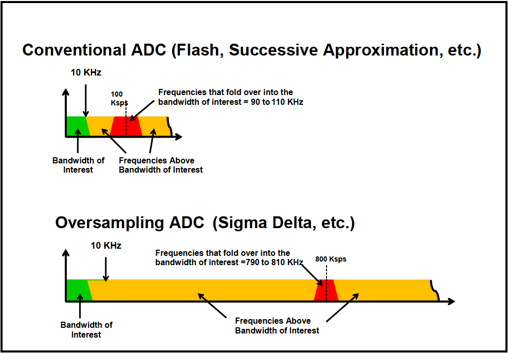
Figure description:
- Figure Title: 516.8A-1b Illustration of sampling rates and out of band "fold over" frequencies for Conventional and Oversampling (Sigma-Delta based data acquisition systems.
- Top Diagram: Conventional ADC (Flash, Successive Approximation, etc.
- Bandwidth of Interest (Green: Up to 10 KHz.
- Sampling Rate: 100 Ksps.
- Frequencies Above Bandwidth of Interest (Yellow: Occupies the region between 10 KHz and the sampling rate.
- Fold-over Region (Red: Frequencies from 90 to 110 KHz fold over into the bandwidth of interest.
- Bottom Diagram: Oversampling ADC (Sigma Delta, etc.
- Bandwidth of Interest (Green: Up to 10 KHz.
- Sampling Rate: 800 Ksps.
- Frequencies Above Bandwidth of Interest (Yellow: Significantly wider region compared to conventional ADC.
- Fold-over Region (Red: Frequencies from 790 to 810 KHz fold over into the bandwidth of interest, pushing the alias risk much higher in the frequency spectrum.
Figure 516.8A-1b Illustration of sampling rates and out of band "fold over" frequencies for Conventional and Oversampling (Sigma-Delta) based data acquisition systems.
516.8 ANNEX A
The example that follows will illustrate initial time domain assessment of a typical transient acceleration time history. Annex B will provide frequency domain and more advanced assessment. Figure 516.8A-2 displays the measurement shock that will be considered for proper processing in both the time and frequency domain. The phenomenon producing the shock has initial high frequency/high energy input, followed by a form of ringing or resonance decay. The measurement shock exists between 617 milliseconds and 1560 milliseconds.
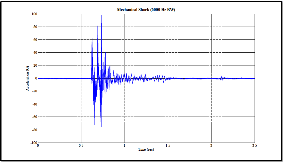
Figure description:
Mechanical Shock (6000 Hz BW
Mechanical Shock (6000 Hz BW
| Time (sec) | Acceleration (G) |
|---|---|
| 0.00 | 0.0 |
| 0.10 | 0.2 |
| 0.20 | -0.1 |
| 0.30 | 0.0 |
| 0.40 | 0.1 |
| 0.50 | 0.0 |
| 0.55 | -0.5 |
| 0.60 | 5.0 |
| 0.61 | 62.0 |
| 0.62 | -35.0 |
| 0.63 | 10.0 |
| 0.64 | -73.0 |
| 0.65 | 18.0 |
| 0.66 | -38.0 |
| 0.67 | 82.0 |
| 0.68 | -25.0 |
| 0.69 | 32.0 |
| 0.70 | -22.0 |
| 0.71 | 98.0 |
| 0.72 | -68.0 |
| 0.73 | 85.0 |
| 0.74 | -75.0 |
| 0.75 | 20.0 |
| 0.76 | 56.0 |
| 0.77 | -18.0 |
| 0.78 | 40.0 |
| 0.80 | -25.0 |
| 0.82 | 18.0 |
| 0.84 | -12.0 |
| 0.86 | 15.0 |
| 0.88 | -8.0 |
| 0.90 | 10.0 |
| 1.00 | 8.0 |
| 1.10 | -6.0 |
| 1.20 | 7.0 |
| 1.30 | -5.0 |
| 1.40 | 4.0 |
| 1.50 | -2.0 |
| 1.60 | 1.0 |
| 1.70 | -0.5 |
| 1.80 | 0.5 |
| 1.90 | -0.2 |
| 2.00 | 0.0 |
| 2.10 | 4.5 |
| 2.15 | -3.0 |
| 2.20 | 1.0 |
| 2.30 | -0.2 |
| 2.40 | 0.1 |
| 2.50 | 0.0 |
Notes: The data values for acceleration are estimated based on visual inspection of the graph's major peaks and oscillations. The shock occurs between approximately 0.6 and 1.5 seconds, with the highest peak reaching nearly 100G at approximately 0.71 seconds.
Figure 516.8A-2. Example acceleration time history.
516.8 ANNEX A
As mentioned in paragraph 1.2, a "simple shock" (refer to Figure 516.8A-3), is defined in terms of three time intervals:
- a. The first time interval; T is usually well defined and occurs prior to the shock where the measurement represents the measurement system noise floor.
- b. The second interval; T is termed the shock duration and is defined as the duration from the zero crossing for the first measurement acceleration “above the instrumentation noise floor" until the perceived "termination" of the shock. This interval contains the interval with the highest concentration of energy, TE, defined |Apk| as the minimum length of time that contains any time history magnitudes exceeding in absolute value (see CF detailed discussion below).
- c. The third time interval; T is the time from the "termination" of the shock until the measurement post signal approaches or reaches levels of the measurement system noise floor. (In general, shocks over reasonable characterization/identification times seldom decay to the levels of the pre-shock noise floor.) This third time interval can be termed the post-shock noise floor that is above, but includes the measurement system noise floor.
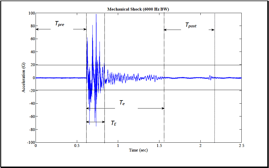
Figure description:
Mechanical Shock Analysis
Mechanical Shock (6000 Hz BW
Annotations
- T_pre (horizontal_interval - position: x from 0 to 0.61)
- T_E (horizontal_interval - position: x from 0.61 to 0.83)
- T_e (horizontal_interval - position: x from 0.61 to 1.56)
- T_post (horizontal_interval - position: x from 1.56 to 2.17)
- Shock start / end of T_pre (vertical_line - position: x = 0.61)
- End of T_E (vertical_line - position: x = 0.83)
- End of T_e / Start of T_post (vertical_line - position: x = 1.56)
- End of T_post (vertical_line - position: x = 2.17)
| Time (sec) | Acceleration (G) |
|---|---|
| 0 | 0 |
| 0.1 | 0.1 |
| 0.2 | -0.2 |
| 0.3 | 0.1 |
| 0.4 | -0.1 |
| 0.5 | 0 |
| 0.6 | 0 |
| 0.61 | 55 |
| 0.62 | -30 |
| 0.63 | 35 |
| 0.64 | -40 |
| 0.65 | 82 |
| 0.66 | -65 |
| 0.68 | 55 |
| 0.7 | 98 |
| 0.71 | -72 |
| 0.72 | -15 |
| 0.73 | 30 |
| 0.74 | -50 |
| 0.75 | 50 |
| 0.76 | -75 |
| 0.78 | 25 |
| 0.8 | 0 |
| 0.85 | 12 |
| 0.9 | -10 |
| 0.95 | 8 |
| 1.0 | -6 |
| 1.1 | 7 |
| 1.2 | -5 |
| 1.3 | 6 |
| 1.4 | -4 |
| 1.5 | 2 |
| 1.55 | 0 |
| 1.6 | 0.5 |
| 1.7 | -0.5 |
| 1.8 | 0.2 |
| 1.9 | -0.3 |
| 2.0 | 0.1 |
| 2.1 | 4 |
| 2.12 | -3 |
| 2.15 | 0 |
| 2.2 | 0.2 |
| 2.3 | -0.1 |
| 2.4 | 0.1 |
| 2.5 | 0 |
Notes: The chart shows a mechanical shock waveform with specific intervals marked. T_pre is the pre-event baseline, T_E represents the duration of the main shock event, T_e is the total event duration including decay, and T_post is the post-event recovery period.
Figure 516.8A-3. Example simple shock time history with segment identification.
In general, for further processing it is convenient, if possible, to select the interval of duration equal to and these intervals should be reasonably comparable or equal in length to . The same amount of "time/amplitude" information is available in all three intervals.
MIL-STD-810H
METHOD 516.8 ANNEX A
516.8 ANNEX A
history magnitudes exceeding in absolute value of . Having established a nominal value for , the synthesis of a representative pulse shall have a tolerance of .
516.8 ANNEX A
range from fmin to ƒ SRS max >1.1f max· From paragraph 1.1 above, the fax relationship to ƒ is defined, however for SRS computation, if F¸ <10ƒSRSÅ the time history must be re-sampled to Fs, >10f SRS max The SRS frequency max spacing in [ƒmin ›1.1ƒmax] is left to the discretion of the analyst, but should not be coarser that one-twelfth octave and, in general, of a proportional band spacing as opposed to a fixed band spacing (proportional band spacing is more in tune with the materiel modal frequency spacing, and results in fewer natural frequencies for processing).
A more complete description of the shock (potentially more useful for shock damage assessment) can be obtained by determining the maximax pseudo-velocity response spectrum. The maximax pseudo-velocity may be plotted on log- log paper with the abscissa as SDOF natural frequency, and the ordinate as pseudo-velocity in units of velocity. Alternatively, a more complete description of the shock (potentially more useful for shock damage assessment) can be obtained by determining the maximax pseudo-velocity response spectrum, and plotting this on four-coordinate paper where, in pairs of orthogonal axes, the maximax pseudo-velocity response spectrum is represented by the ordinate, with the undamped natural frequency being the abscissa, and the maximax absolute acceleration along with maximax pseudo-displacement plotted in a pair of orthogonal axes, all plots having the same abscissa (SDOF natural frequency). This form of a pseudo-velocity SRS plot, as seen in Figure 516.8A-4, is widely accepted in Civil Engineering earthquake ground motion specifications, but historically has not been as common for mechanical shock display or specification.
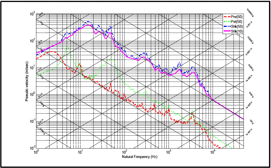
Figure description:
Shock Response Spectra
Shock Response Spectra Tripartite Plot
Legend
- Pre(50 — color: red; symbol: Dashed line
- Pst(50 — color: green; symbol: Dotted line
- Shk(50 — color: blue; symbol: Dash-dot line
- Shk(10 — color: magenta; symbol: Solid line
Annotations
- Displacement lines (slope +1 (reference_line - position: Diagonal lines labeled with values like 50 in, 10 in, 1 in, etc.))
- Acceleration lines (slope -1 (reference_line - position: Diagonal lines labeled with values like 0.001 g, 0.01 g, 0.1 g, 100 g, etc.))
| Natural Frequency (Hz) | Pre(50 (in/sec)) | Pst(50 (in/sec)) | Shk(50 (in/sec)) | Shk(10 (in/sec)) |
|---|---|---|---|---|
| 1.0 | 30.0 | 6.5 | 35.0 | 35.0 |
| 1.5 | 42.0 | 8.0 | 45.0 | 45.0 |
| 2.0 | 45.0 | 10.0 | 65.0 | 65.0 |
| 3.0 | 35.0 | 18.0 | 150.0 | 120.0 |
| 4.0 | 25.0 | 30.0 | 180.0 | 150.0 |
| 5.0 | 18.0 | 45.0 | 200.0 | 160.0 |
| 7.0 | 10.0 | 15.0 | 180.0 | 180.0 |
| 10.0 | 13.0 | 6.5 | 350.0 | 250.0 |
| 15.0 | 5.5 | 4.0 | 500.0 | 400.0 |
| 20.0 | 4.0 | 5.5 | 380.0 | 320.0 |
| 30.0 | 2.5 | 8.0 | 280.0 | 220.0 |
| 40.0 | 1.8 | 15.0 | 220.0 | 180.0 |
| 50.0 | 2.8 | 20.0 | 380.0 | 280.0 |
| 60.0 | 1.5 | 18.0 | 250.0 | 180.0 |
| 80.0 | 1.2 | 8.0 | 80.0 | 65.0 |
| 100.0 | 0.8 | 3.5 | 40.0 | 35.0 |
| 150.0 | 0.5 | 1.5 | 28.0 | 22.0 |
| 200.0 | 0.4 | 1.0 | 30.0 | 25.0 |
| 300.0 | 0.3 | 0.8 | 40.0 | 25.0 |
| 400.0 | 0.35 | 0.5 | 20.0 | 18.0 |
| 500.0 | 0.22 | 0.6 | 12.0 | 10.0 |
| 700.0 | 0.2 | 0.35 | 8.0 | 6.0 |
| 1000.0 | 0.22 | 0.22 | 7.0 | 6.0 |
| 1500.0 | 0.1 | 0.15 | 18.0 | 10.0 |
| 2000.0 | 0.09 | 0.1 | 12.0 | 8.0 |
| 3000.0 | 0.1 | 0.18 | 12.0 | 8.0 |
| 4000.0 | 0.18 | 0.08 | 7.0 | 6.0 |
| 5000.0 | 0.12 | 0.06 | 3.0 | 2.5 |
| 7000.0 | 0.05 | 0.03 | 1.2 | 1.1 |
| 10000.0 | 0.015 | 0.018 | 0.7 | 0.7 |
| 20000.0 | 0.007 | 0.3 | 0.3 | |
| 30000.0 | 0.18 | 0.18 | ||
| 50000.0 | 0.12 | 0.12 |
Notes: The figure is a tripartite log-log plot showing Pseudo Velocity (in/sec vs. Natural Frequency (Hz. It features secondary diagonal axes for Displacement (in and Acceleration (g. Data points are sampled across the frequency range and are approximate.))))
Figure 516.8A-4. Maximax pseudo-velocity SRS estimates for shock and noise floor segments.
The maximax pseudo-velocity at a particular SDOF undamped natural frequency is thought to be more representative of the damage potential for a shock since it correlates with stress and strain in the elements of a single degree of freedom system (paragraph 7.1, references e and f). In the laboratory testing to meet a given specification with undesignated Q, use a Q value of 10 and a second Q value of 50 for comparison in the processing (see Figure 516.8A- 4). Using two Q values, a damped value and a value corresponding to light damping provides an analyst with information on the potential spread of maximum materiel response. Recommend the maximax absolute acceleration SRS be the primary method of display for the shock, with the maximax pseudo-velocity SRS the secondary method
MIL-STD-810H
METHOD
516.8 ANNEX A
of display. This is useful in cases in which it is desirable to be able to correlate damage of simple systems with the shock. Two additional recommendations related to the validity of the measurement are as follows:
a. A pre-shock SRS of the measurement system noise floor over interval should be computed along with the return to noise floor interval , i.e., post-shock noise floor, and displayed on the same plot. These noise SRSs help to confirm the overall validity of the measurement if the "Pre" and "Post" times allow adequate accuracy for the SRS estimates, i.e., SRS estimates over very short time segments may not provide representative maximax SRS amplitudes at low natural frequencies. These SRS estimates should be computed at the Q=50 damping value (see Figure 516.8A-4). Refer to Annex B, paragraph 3 for additional guidance on establishing criteria for defining the noise floor.
- b. For the shock segment, both the maximum positive and maximum negative acceleration and pseudo- velocity SRS estimates should be plotted for a minimum Q value of 10 over the frequency range for which the shock SRS values are displayed (see Figure 516.8A-5). The positive and negative SRS estimates should be very similar in nature as discussed in paragraph 1.4.2 and illustrated through example in Figures 516.8A-5&6. The low Q value should be able to detect acceleration time history anomalies similar to the time history integration. If positive and negative SRS maximax values are disparate, this could be an indicator of potential measurement system signal conditioning problems.
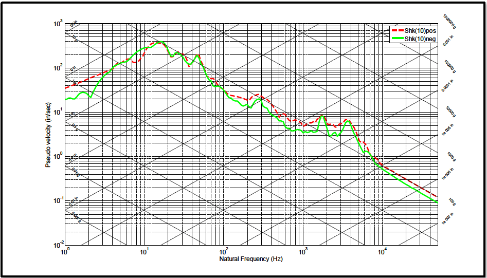
Figure description:
Legend
- Shk(10pos — color: red; symbol: Dashed line
- Shk(10neg — color: green; symbol: Solid line
Annotations
- Acceleration (g lines (text_label - position: Diagonal grid lines sloping up to the right ranging from 0.001g to 1,000,000g))
- Displacement (in lines (text_label - position: Diagonal grid lines sloping down to the right ranging from 1000in to 1e-07in))
| Natural Frequency (Hz) | Shk(10pos Pseudo velocity (in/sec)) | Shk(10neg Pseudo velocity (in/sec)) |
|---|---|---|
| 1.0 | 40.0 | 20.0 |
| 1.5 | 55.0 | 28.0 |
| 2.0 | 70.0 | 22.0 |
| 3.0 | 85.0 | 45.0 |
| 4.0 | 110.0 | 90.0 |
| 5.0 | 150.0 | 120.0 |
| 7.0 | 180.0 | 180.0 |
| 8.0 | 140.0 | 220.0 |
| 10.0 | 180.0 | 280.0 |
| 12.0 | 300.0 | 380.0 |
| 15.0 | 380.0 | 380.0 |
| 20.0 | 250.0 | 250.0 |
| 30.0 | 180.0 | 180.0 |
| 45.0 | 180.0 | 180.0 |
| 50.0 | 120.0 | 110.0 |
| 70.0 | 55.0 | 50.0 |
| 100.0 | 30.0 | 28.0 |
| 150.0 | 25.0 | 20.0 |
| 200.0 | 18.0 | 15.0 |
| 300.0 | 25.0 | 20.0 |
| 400.0 | 18.0 | 15.0 |
| 500.0 | 10.0 | 8.0 |
| 700.0 | 8.0 | 6.0 |
| 800.0 | 6.5 | 5.0 |
| 1000.0 | 5.0 | 4.0 |
| 1500.0 | 8.0 | 6.0 |
| 2000.0 | 5.0 | 4.0 |
| 3000.0 | 4.5 | 3.5 |
| 4000.0 | 7.0 | 6.0 |
| 5000.0 | 4.0 | 3.0 |
| 7000.0 | 1.5 | 1.2 |
| 10000.0 | 0.8 | 0.6 |
| 20000.0 | 0.3 | 0.25 |
| 50000.0 | 0.12 | 0.09 |
Notes: The chart is a tripartite response spectrum plot showing pseudo velocity versus natural frequency on a log-log scale, with supplemental diagonal axes for displacement and acceleration.
Figure 516.8A-5. Shock maximum and minimum pseudo-velocity SRS estimates.
MIL-STD-810H METHOD 516.8 ANNEX A
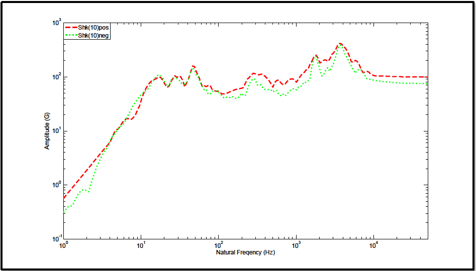
Figure description:
Legend
- Shk(10pos — color: red; symbol: Dashed line
- Shk(10neg — color: green; symbol: Dotted line
| Natural Frequency (Hz) | Shk(10pos Amplitude (G)) | Shk(10neg Amplitude (G)) |
|---|---|---|
| 1.0 | 0.58 | 0.32 |
| 1.5 | 1.14 | 0.65 |
| 2.0 | 2.10 | 0.78 |
| 5.0 | 11.50 | 10.20 |
| 10.0 | 32.00 | 44.00 |
| 15.0 | 95.00 | 105.00 |
| 20.0 | 72.00 | 68.00 |
| 30.0 | 105.00 | 82.00 |
| 45.0 | 155.00 | 135.00 |
| 65.0 | 72.00 | 52.00 |
| 100.0 | 52.00 | 48.00 |
| 200.0 | 65.00 | 44.00 |
| 280.0 | 115.00 | 95.00 |
| 550.0 | 88.00 | 54.00 |
| 1000.0 | 82.00 | 68.00 |
| 1800.0 | 245.00 | 195.00 |
| 2500.0 | 195.00 | 115.00 |
| 3800.0 | 415.00 | 395.00 |
| 6000.0 | 185.00 | 125.00 |
| 10000.0 | 105.00 | 88.00 |
| 20000.0 | 100.00 | 80.00 |
| 40000.0 | 100.00 | 78.00 |
Notes: The chart uses logarithmic scales for both axes. The X-axis represents Natural Frequency in Hertz (Hz and the Y-axis represents Amplitude in Gs.)
Figure 516.8A-6. Shock maximum and minimum acceleration SRS estimates.
516.8 ANNEX A
or tests. The best summary option is generally dependent on the size of sample. Processed results from the SRS or ESD are typically logarithmically transformed to provide estimates that tend to be more normally distributed, e.g., estimates in dB. This transformation is important since often very few estimates are available from a test series, and the probability distribution of the untransformed estimates cannot be assumed to be normally distributed. In virtually all cases, combination of processed results will fall under the category of small sample statistics, and need to be considered with care with other parametric or less powerful nonparametric methods of statistical analysis. Annex C addresses the appropriate techniques for the statistical combination of processed test results as a function of the size of the sample and provides an example.
516.8 ANNEX B METHOD 516.8, ANNEX B GUIDELINES FOR ADDITIONAL SHOCK TIME HISTORY VALIDATION AND PROCESSING
516.8 ANNEX B
computing the average at each time point. Usually, plotting these rms levels leads to simple identification of . Specifying the normalized random error for the rms estimate can enhance this procedure.
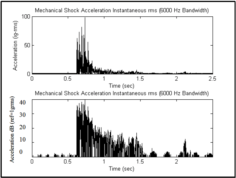
Figure description:
Mechanical Shock Acceleration Data
Mechanical Shock Acceleration Instantaneous rms (6000 Hz Bandwidth
| Time (sec) | Acceleration (g-rms) |
|---|---|
| 0.0 | 0.0 |
| 0.2 | 0.0 |
| 0.4 | 0.0 |
| 0.5 | 0.0 |
| 0.6 | 0.0 |
| 0.63 | 62.0 |
| 0.65 | 42.0 |
| 0.68 | 81.0 |
| 0.72 | 68.0 |
| 0.75 | 98.0 |
| 0.8 | 45.0 |
| 0.85 | 30.0 |
| 0.9 | 22.0 |
| 1.0 | 11.0 |
| 1.2 | 8.0 |
| 1.5 | 4.0 |
| 1.8 | 2.0 |
| 2.0 | 1.0 |
| 2.1 | 5.0 |
| 2.2 | 1.0 |
| 2.5 | 0.5 |
Mechanical Shock Acceleration Instantaneous rms (6000 Hz Bandwidth
| Time (sec) | Acceleration dB (ref=1grms) |
|---|---|
| 0.0 | -3.0 |
| 0.2 | -2.0 |
| 0.4 | -2.0 |
| 0.5 | -3.0 |
| 0.6 | -1.0 |
| 0.63 | 36.0 |
| 0.65 | 33.0 |
| 0.68 | 39.0 |
| 0.72 | 37.0 |
| 0.75 | 42.0 |
| 0.8 | 34.0 |
| 0.85 | 30.0 |
| 0.9 | 27.0 |
| 1.0 | 21.0 |
| 1.2 | 18.0 |
| 1.5 | 12.0 |
| 1.8 | 2.0 |
| 2.0 | 0.0 |
| 2.1 | 11.0 |
| 2.2 | 0.0 |
| 2.5 | -1.0 |
Notes: The plots represent a high-frequency transient mechanical shock. The data provided in the tables are representative samples that capture the envelope and significant peak features of the signals.
Figure 516.8B-3. Shock time history instantaneous root-mean-square.
This error is given by for the bandwidth and the averaging time. A 95 percent confidence interval is defined by . For , then . Estimating both the measurement system noise floor and post-shock_noise floor levels (standard deviations) for a specified normalized random error, e.g., 0.025 , computing the 95 percent confidence intervals and determining the degree of overlap of the measurement system noise floor and post-shock noise floor confidence intervals can provide an analytical criterion for specifying the ed of a shock. Excessive noise that may not be Gaussian in form in the post-shock noise floor may be an indication of a degraded instrumentation signal conditioning system as a result of the shock, e.g., broken accelerometer sensing element, amplifier slew rate exceeded, etc. In this case, the post-shock integrity of the measurement system needs to be validated (see paragraph 4 below).
If such computation and subsequent displays are not available, the assessment for the end of the shock, and beginning of the post-shock noise floor can be determined based on examination of a representative sample of the positive and negative peaks in the time history (usually starting from the end of the measurement and avoiding single spurious "noise spikes") without regard to sign. In this case, the maximum peak (positive or negative) can be estimated in absolute units, and then a -20 dB, -30 dB, and -40 dB level down from the validated peak , estimated by for the desired dB decrement, and representing either a positive or negative peak.
Because of the need to balance the normalized random error with the normalized bias error to determine optimum averaging times, it is not recommended that the instantaneous rms values be smoothed through short-time-averaging.
MIL-STD-810H METHOD
516.8 ANNEX B
516.8 ANNEX B
For validation purposes, the ESD estimate should display proper frequency domain characteristics. In particular, the DC region should be rolled-off if the DC time history component has been removed, and the maximum bandwidth levels should be rolled-off if aliasing is not present. If the maximum bandwidth levels show an increase, it is quite possible that aliasing is present provided the time history has not been previously filtered. An ESD estimate needs to be computed on a high-passed time history that has been not bandlimited by digital filtering in any way.
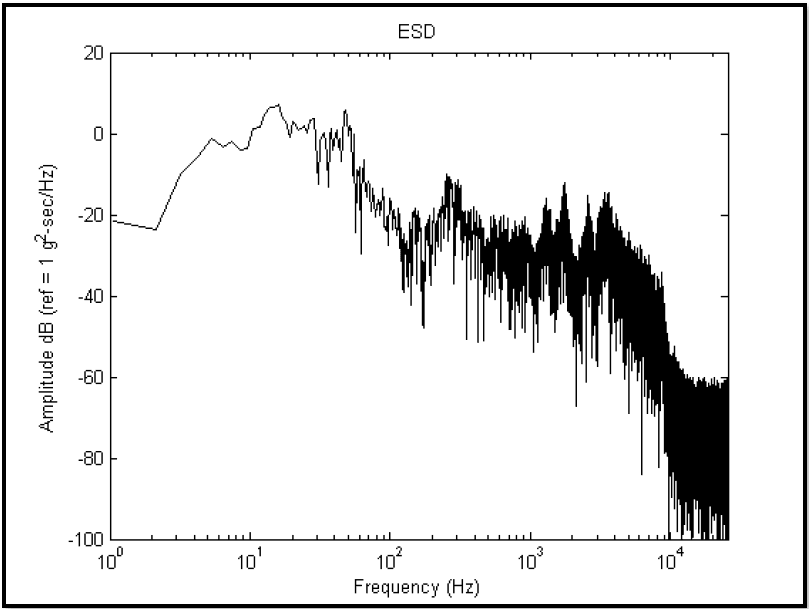
Figure description:
ESD
ESD
| Frequency (Hz) | Amplitude dB (ref = 1 g^2-sec/Hz) |
|---|---|
| 1.0 | -21.4 |
| 1.5 | -22.5 |
| 2.1 | -23.4 |
| 3.1 | -9.6 |
| 4.4 | -4.4 |
| 5.4 | -1.2 |
| 6.9 | -3.1 |
| 8.3 | -2.3 |
| 10.4 | 1.3 |
| 13.5 | 6.4 |
| 16.5 | 7.3 |
| 18.2 | 3.3 |
| 20.2 | -0.6 |
| 24.8 | 3.0 |
| 30.5 | 3.9 |
| 34.0 | -7.2 |
| 41.5 | 0.8 |
| 48.5 | 6.0 |
| 55.4 | -1.1 |
| 65.6 | -23.8 |
| 102.3 | -24.8 |
| 155.4 | -33.9 |
| 256.4 | -9.6 |
| 300.0 | -13.6 |
| 510.5 | -23.6 |
| 985.4 | -30.4 |
| 1200.0 | -17.8 |
| 1780.0 | -12.4 |
| 2540.0 | -24.0 |
| 3500.0 | -14.6 |
| 4200.0 | -17.4 |
| 8500.0 | -34.8 |
| 10000.0 | -54.3 |
| 15000.0 | -60.8 |
| 25000.0 | -63.4 |
Notes: The chart is a semi-log plot of Energy Spectral Density (ESD. The x-axis (Frequency is on a logarithmic scale, while the y-axis (Amplitude is on a linear scale in decibels. The data is highly noisy, especially at higher frequencies where it exhibits a broad noise floor starting around 10,000 Hz.)))
Figure 516.8B-6. Shock ESD estimate.
516.8 ANNEX C
NOTE: A “random design” allows the independent variable to vary among estimates and requires principles of distribution-free non-parametric regression techniques to assess the relationship among the estimates.
- b. The uncertainty or error in individual estimate processing (random or bias processing error) does not significantly affect limit considerations.
NOTE: For Fourier based estimates such as ASD, ESD or FS, the estimate accuracy will be defined in terms of statistical degrees of freedom. For example, a basic periodogram estimate has two statistical degrees of freedom, but through block averaging (in time) using the Welch procedure or averaging of adjacent frequencies (in frequency), the statistical degrees of freedom in the estimate can be increased with subsequent decrease in estimate random error, but potential increase in corresponding estimate bias error. It is important in making estimates that the processing error be minimized (or optimized) in some sense through either extending (if possible) the stationary random time history processing length, or by increasing the estimate bandwidth by frequency averaging. In the case of non-Fourier based estimates such as the SRS, there is little guidance on processing bandwidth selection, except that based upon physical considerations for single-degree-of-freedom systems. In these cases, recommend selection of different damping factors along with bandwidths, and comparing the limits.
- c. Individual estimates from a given measurement are uncorrelated with one another, i.e., there is no serial correlation with respect to the independent variable.
NOTE: For Fourier based estimates, this assumption is usually fulfilled because of the “orthogonality” of the Fourier transform. For non-Fourier based estimates, e.g., SRS, some serial correlation in estimates is unavoidable.
- d. Transformed estimates often are more in line with the assumptions behind the limit determination procedures. For example, using a logarithm transform to yield the estimates in dB will generally leave the estimate set at a given frequency closer to being normally distributed.
- e. Near “optimal limit estimates” may be determined potentially by reprocessing available time trace information through change in the spacing of the independent variable, i.e., the analysis bandwidth. For the case of prediction, this would mean interpolation of the given prediction estimates.
- f. Parametric and non-parametric based limit estimates are available. The analyst should select one or more limit estimates that best aligns with (a) the desired interpretation of the limit assessment, and (b) the character of the set of “similar estimates”.
516.8 ANNEX C
for a single bandwidth, and that estimates among bandwidths are independent, so that each bandwidth under consideration may be processed individually, and the results summarized on one plot over the entire bandwidth as a function of frequency. For
Yi = log10(xi) i = 1,2 N
Mean estimate for true mean, μy is given by
1 N my Σ yi N i=1
and the unbiased estimate of the standard deviation for the true standard deviation is given by
516.8 ANNEX C
| N | γ = 0.50 | γ = 0.90 | γ = 0.95 | ||||||
|---|---|---|---|---|---|---|---|---|---|
| β = 0.90 | β = 0.95 | β = 0.99 | β = 0.90 | β = 0.95 | β = 0.99 | β = 0.90 | β = 0.95 | β = 0.99 | |
| 3 | 1.50 | 1.94 | 2.76 | 4.26 | 5.31 | 7.34 | 6.16 | 7.66 | 10.55 |
| 4 | 1.42 | 1.83 | 2.60 | 3.19 | 3.96 | 5.44 | 4.16 | 5.14 | 7.04 |
| 5 | 1.38 | 1.78 | 2.53 | 2.74 | 3.40 | 4.67 | 3.41 | 4.20 | 5.74 |
| 6 | 1.36 | 1.75 | 2.48 | 2.49 | 3.09 | 4.24 | 3.01 | 3.71 | 5.06 |
| 7 | 1.35 | 1.73 | 2.46 | 2.33 | 2.89 | 3.97 | 2.76 | 3.40 | 4.64 |
| 8 | 1.34 | 1.72 | 2.44 | 2.22 | 2.75 | 3.78 | 2.58 | 3.19 | 4.35 |
| 9 | 1.33 | 1.71 | 2.42 | 2.13 | 2.65 | 3.64 | 2.45 | 3.03 | 4.14 |
| 10 | 1.32 | 1.70 | 2.41 | 2.07 | 2.57 | 3.53 | 2.35 | 2.91 | 3.98 |
| 11 | 1.32 | 1.70 | 2.40 | 2.01 | 2.50 | 3.44 | 2.28 | 2.82 | 3.85 |
| 12 | 1.32 | 1.69 | 2.39 | 1.97 | 2.45 | 3.37 | 2.21 | 2.74 | 3.75 |
| 13 | 1.31 | 1.69 | 2.39 | 1.93 | 2.40 | 3.31 | 2.16 | 2.67 | 3.66 |
| 14 | 1.31 | 1.68 | 2.38 | 1.90 | 2.36 | 3.26 | 2.11 | 2.61 | 3.58 |
| 15 | 1.31 | 1.68 | 2.38 | 1.87 | 2.33 | 3.21 | 2.07 | 2.57 | 3.52 |
| 16 | 1.31 | 1.68 | 2.38 | 1.84 | 2.30 | 3.17 | 2.03 | 2.52 | 3.46 |
| 17 | 1.31 | 1.68 | 2.37 | 1.82 | 2.27 | 3.14 | 2.00 | 2.49 | 3.41 |
| 18 | 1.30 | 1.67 | 2.37 | 1.80 | 2.25 | 3.11 | 1.97 | 2.45 | 3.37 |
| 19 | 1.30 | 1.67 | 2.37 | 1.78 | 2.23 | 3.08 | 1.95 | 2.42 | 3.33 |
| 20 | 1.30 | 1.67 | 2.37 | 1.77 | 2.21 | 3.05 | 1.93 | 2.40 | 3.30 |
| 21 | 1.30 | 1.67 | 2.36 | 1.75 | 2.19 | 3.03 | 1.91 | 2.37 | 3.26 |
| 22 | 1.30 | 1.67 | 2.36 | 1.74 | 2.17 | 3.01 | 1.89 | 2.35 | 3.23 |
| 23 | 1.30 | 1.67 | 2.36 | 1.72 | 2.16 | 2.99 | 1.87 | 2.33 | 3.21 |
| 24 | 1.30 | 1.67 | 2.36 | 1.71 | 2.15 | 2.97 | 1.85 | 2.31 | 3.18 |
| 25 | 1.30 | 1.67 | 2.36 | 1.70 | 2.13 | 2.95 | 1.84 | 2.29 | 3.16 |
| 26 | 1.30 | 1.66 | 2.36 | 1.69 | 2.12 | 2.94 | 1.82 | 2.28 | 3.14 |
| 27 | 1.30 | 1.66 | 2.35 | 1.68 | 2.11 | 2.92 | 1.81 | 2.26 | 3.12 |
| 28 | 1.30 | 1.66 | 2.35 | 1.67 | 2.10 | 2.91 | 1.80 | 2.25 | 3.10 |
| 29 | 1.29 | 1.66 | 2.35 | 1.66 | 2.09 | 2.90 | 1.79 | 2.23 | 3.08 |
| 30 | 1.29 | 1.66 | 2.35 | 1.66 | 2.08 | 2.88 | 1.78 | 2.22 | 3.06 |
| 32 | 1.29 | 1.66 | 2.35 | 1.64 | 2.06 | 2.86 | 1.76 | 2.20 | 3.03 |
| 34 | 1.29 | 1.66 | 2.35 | 1.63 | 2.05 | 2.84 | 1.74 | 2.18 | 3.01 |
| 36 | 1.29 | 1.66 | 2.35 | 1.62 | 2.03 | 2.82 | 1.72 | 2.16 | 2.98 |
| 38 | 1.29 | 1.66 | 2.35 | 1.61 | 2.02 | 2.81 | 1.71 | 2.14 | 2.96 |
| 40 | 1.29 | 1.66 | 2.35 | 1.60 | 2.01 | 2.79 | 1.70 | 2.13 | 2.94 |
| 42 | 1.29 | 1.66 | 2.34 | 1.59 | 2.00 | 2.78 | 1.69 | 2.11 | 2.92 |
| 44 | 1.29 | 1.66 | 2.34 | 1.58 | 1.99 | 2.77 | 1.67 | 2.10 | 2.91 |
| 46 | 1.29 | 1.66 | 2.34 | 1.57 | 1.98 | 2.76 | 1.66 | 2.09 | 2.89 |
| 48 | 1.29 | 1.66 | 2.34 | 1.57 | 1.97 | 2.74 | 1.65 | 2.08 | 2.88 |
| 50 | 1.29 | 1.65 | 2.34 | 1.56 | 1.97 | 2.73 | 1.65 | 2.07 | 2.86 |
| 55 | 1.28 | 1.64 | 2.33 | 1.54 | 1.94 | 2.70 | 1.62 | 2.04 | 2.83 |
| 60 | 1.28 | 1.64 | 2.33 | 1.53 | 1.93 | 2.68 | 1.60 | 2.02 | 2.80 |
| 65 | 1.28 | 1.64 | 2.33 | 1.52 | 1.91 | 2.67 | 1.59 | 2.00 | 2.78 |
| 70 | 1.28 | 1.64 | 2.33 | 1.51 | 1.90 | 2.65 | 1.58 | 1.99 | 2.76 |
| 75 | 1.28 | 1.64 | 2.33 | 1.50 | 1.89 | 2.64 | 1.57 | 1.97 | 2.74 |
| 80 | 1.28 | 1.64 | 2.33 | 1.49 | 1.88 | 2.63 | 1.56 | 1.96 | 2.73 |
| 85 | 1.28 | 1.64 | 2.33 | 1.48 | 1.88 | 2.62 | 1.55 | 1.95 | 2.71 |
| 90 | 1.28 | 1.64 | 2.33 | 1.48 | 1.87 | 2.61 | 1.54 | 1.94 | 2.70 |
| 95 | 1.28 | 1.64 | 2.33 | 1.47 | 1.86 | 2.60 | 1.53 | 1.93 | 2.69 |
| 100 | 1.28 | 1.64 | 2.33 | 1.47 | 1.86 | 2.60 | 1.52 | 1.92 | 2.68 |
| 500 | 1.28 | 1.64 | 2.33 | 1.36 | 1.74 | 2.44 | 1.38 | 1.76 | 2.47 |
| 1000 | 1.28 | 1.64 | 2.33 | 1.34 | 1.71 | 2.41 | 1.35 | 1.73 | 2.43 |
| ∞ | 1.28 | 1.64 | 2.33 | 1.34 | 1.71 | 2.41 | 1.35 | 1.73 | 2.43 |
MIL-STD-810H METHOD
516.8 ANNEX C
The table (Table 516.8C-I) from paragraph 6.1, reference b, contains the k value for selected N, ẞ, Y. In general this method of estimation should not be used for small N with values of ẞ and y close to 1 since it is likely the assumption of the normality of the logarithm transform of the estimates will be violated.