527.2-6 MDOF VSD METHODS
6.1 Referenced Documents
- a. NATO STANAG 4370, Environmental Testing, Allied Environmental Conditions and Test Publication (AECTP) 200, Mechanical Environmental Testing, Category 240.
- b. International Test Operations Procedure (ITOP) 01-1-050, "Development of Laboratory Vibration Test Schedules", 6 June 1997, DTIC AD No. B227368.
- c. International Test Operations Procedure (ITOP) 01-2-601, "Laboratory Vibration Schedules", 25 January 1999. DTIC AD No. B238288.
- d. Bendat, Julius S. and Allan G. Piersol, Random Data Analysis and Measurement Procedures, 3rd Edition, John Wiley & Sons, Inc., New York, 2000.
- e. Handbook for Dynamic Data Acquisition and Analysis, IEST-RD-DTE012.2; Institute of Environmental Sciences and Technology, Arlington Place One, 2340 S. Arlington Heights Road, Suite 100, Arlington Heights, IL 60005-4516; Institute of Environmental Sciences and Technology Website.
- f. Fitz-Coy, Norman and Hale, Michael T., “On the Use of Linear Accelerometers in Six-DOF Laboratory Motion Replication: A Unified Time-Domain Analysis”, Proceedings of the 76th Shock and Vibration Symposium, Nov. 2005. Shock & Vibration Exchange (SAVE), 1104 Arvon Road, Arvonia, VA 23004.
- g. Underwood, Marcos A. and Keller, Tony, “Applying Coordinate Transformations to Multi-DOF Shaker Control”, Sound and Vibration, January 2006, Sound and Vibration Website.
- h. Shock and Vibration Handbook, 5th Edition, Edited by Cyril M. Harris and Allan G. Piersol, McGraw-Hill, New York NY, 2002.
- i. Smallwood, David O., “Multiple Shaker Random Vibration Control – An Update”, SAND 98-2044C.
MIL-STD-810H
METHOD 527.2
- j. Smallwood, David, Multiple-Input Multiple-Output (MIMO) Linear Systems Extreme Inputs/Outputs. Shock and Vibration 14 (2007) 107-131; IOS Press, Inc.
- k. Hale, Michael T., “Consideration of Global Error Metrics in the Conduct of MDOF Motion Replication”, Proceedings of the 77th Shock and Vibration Symposium, Nov. 2006; Shock & Vibration Exchange (SAVE), 1104 Arvon Road, Arvonia, VA 23004.
- Underwood, Marcos A. and Keller, Tony, "Using the Spectral Density Matrix to Determine Ordinary, Partial, and Multiple Coherence", Proceedings of the 77th Shock & Vibration Symposium, October, 2006; Monterey, California.
- m. Underwood, Marcos A., "Multi-Exciter Testing Applications: Theory and Practice", Proceedings – Institute of Environmental Sciences and Technology, April 2002.
- n. Plummer, A.R., “Control Techniques for Structural Testing: A Review”, Proc. IMechE Vol. 221 Part I: J. Systems and Control Engineering, 2007.
- o. Welch, P.D., "The use of fast Fourier transform for the estimation of power spectra: A method based on time averaging over short, modified periodograms", IEEE Transactions on Audio and Electroacoustics, Vol. AU-15, No. 2, June 1967.
- p. Fitz-Coy, N., Hale, M. and Nagabhushan, V., "Benefits and Challenges of Over-Actuated Excitation Systems", Shock and Vibration Journal, Volume 17, Number 3 / 2010.
- q. Hale, Michael T., "Spectral Density Matrix Transformations", Journal of the IEST, V. 60, No. 1, pp 17-26, 2017.
527.2-6.1 Options Considered
Having reviewed the data acquisition and analysis requirements, this section is dedicated to defining the steps for two candidate MDOF VSD methodologies17. Method I is processed in the SDM domain and Method II conducts averaging steps in the Cholesky Domain. An example follows in paragraph 6.3.
6.1.1 Method I
The following is a 10 step outline of Method I (SDM Domain) MDOF VSD:
Step 1 Prepare to convert field measurements into motion DOFs.
MIL-STD-810H METHOD
6.1.2 Method II
The following is a 10 step outline of Method II (Cholesky Domain) MDOF VSD:
Step 1-4 Correlate directly to Method I Outline.
- Step 5 Perform a Cholesky decomposition on the individual SDM associated with each Run in the mission scenario.
Since each individual Run was based on a physical event, the individual SDM’s should be positive definite, thereby making the Cholesky decomposition possible. (Recall all Runs would have been tested to verify each was positive definite or corrected as required per Step 3).
Either organize all of the lower triangular matrices resulting from the Cholesky decomposition for the Runs of interest into a logical structure or merge them into one file of known matrix structure such as [CHOL_Run1,CHOL_Run2 CHOL_RunN] to optimize the conduct basic statistics.
- Step 6 Compute a weighted average Lower Triangular Matrix of the N Cholesky decompositions of Step 5.
The weighting factor on the average will be directly correlated to the mission scenario identified in Step 1. Note that the resulting average will still consist of positive eigenvalues implying that when converted back into the SDM format that the result will be positive definite.
Once converted back into the SDM domain, the resulting CSD terms will generally be highly comparable to the average CSD values computed in Step 6 of Method I. However, the rms levels
MIL-STD-810H METHOD
6.2 Related Documents
Egbert, Herbert W. “The History and Rationale of MIL-STD-810 (Edition 2)”, January 2010; Institute of Environmental Sciences and Technology, Arlington Place One, 2340 S. Arlington Heights Road, Suite 100, Arlington Heights, IL 60005-4516.
(Copies of Department of Defense Specifications, Standards, and Handbooks, and International Standardization Agreements are available online at https://assist.dla mil.
Requests for other defense-related technical publications may be directed to the Defense Technical Information Center (DTIC), ATTN: DTIC-BR, Suite 0944, 8725 John J. Kingman Road, Fort Belvoir VA 22060-6218, 1-800-225-3842 (Assistance--selection 3, option 2), http://www.dtic.mil/dtic/; and the National Technical Information Service (NTIS), Springfield VA 22161, 1-800-553-NTIS (6847), http://www ntis.gov/.
Downloaded from https://www.everyspec.com
MIL-STD-810H METHOD 527.2
(This page is intentionally blank.)
MIL-STD-810H METHOD
527.2-6.2 Example
- a. To illustrate the process discussed above, a simple example was derived (Method I is addressed first). Using an available wheeled vehicle, the input to an onboard missile storage rack was instrumented as shown in Figure 4. The transducer at the center of Figure 4 was placed at the user defined origin, position [0,0,0], in terms of a Cartesian coordinate system. In a traditional right hand orientation, the forward direction of the vehicle was defined as the positive x-axis, towards the vehicle driver's side was considered positive y-axis, and through the vehicle roof was considered the positive z-axis. All transducers are referenced in terms of their relative placement to the origin as discussed previously in the acceleration transformation section of this Annex.
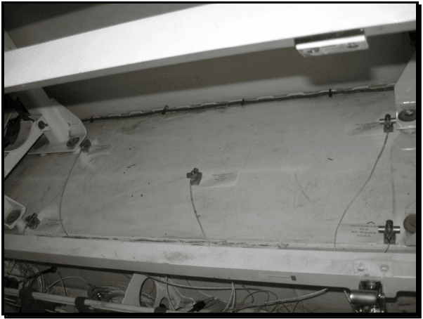
Figure description:
- Subject: Transducer placement on a missile rack (input side for a TOW system on a Stryker vehicle.
- Key Entities:
- Transducers: Five sensors mounted at various points on a flat, white panel.
- Identification Labels: Small white tags located next to each transducer. Visible text includes "TOW on Stryker S-DCR" and "Rack - Alt Roadside."
- Wiring: Thin gray cables connecting to each sensor and routed toward the bottom of the frame.
- Structural Frame: The panel is mounted within a heavy-duty white metal rack assembly.
Figure 4. Transducer placement (input to missile rack).
b. Method I Example
- (1) Having established a clear coordinate system definition, the key parameters discussed in Step 1 are identified. In distance units of inches, the positions of the four corner accelerometer locations used in this example are defined as:
MIL-STD-810H
METHOD 527.2 ANNEX E
r1=[−17,−6,0]', r2=[−17,6,0]', r3 =[17,—6,0]', r4 = [17,6,0]', which in skew symmetric form are:
0 0 -6 0 0 6 0 0 -6 0 0 6
[P] = 0 0 17,[2] 0 0 [17],["} ]* = | 0 0-17[Pr] 0 0 -17
6 -17 0 -6-17 0 6 17 0 -6 17 0
For convenience, the instrumentation team placed the tri-axial transducers such that the channel used to measure the y-axis motion was actually 180 degrees out of phase with respect to the referenced coordinate system. This issue is addressed by simply defining row selection vectors as ex = [1,0,0], e] = [0,−1,0], e =[0,0,1]. Matrix T and matrix T may now be computed as per the discussion in paragraph 4.4.1.1 as:
1 00 0 0 6
0-10 0 0 17
0 0 1-6 17 0
100 0 0 -6
0-1 0 1000 0 0 17
00 6 17 0 Ta 10 0 0 0 6
0-1 0 0 0 -17
00 1-6-17 0
100 0 0 -6
0-10 0 0 -17
0 0 1 6 -17 0
| 0.2500 | 0 | 0 | 0.2500 | 0 | 0 | 0.2500 | 0 | 0 | 0.2500 | 0 | 0 |
| 0 | -0.2500 | 0 | 0 | -0.2500 | 0 | 0 | -0.2500 | 0 | 0 | -0.2500 | 0 |
| 0 | 0 | 0.2500 | 0 | 0 | 0.2500 | 0 | 0 | 0.2500 | 0 | 0 | 0.2500 |
| 0 | 0 | -0.0417 | 0 | 0 | 0.0417 | 0 | 0 | -0.0417 | 0 | 0 | 0.0417 |
| 0 | 0 | 0.0147 | 0 | 0 | 0.0147 | 0 | 0 | -0.0147 | 0 | 0 | -0.0147 |
| 0.0046 | 0.0131 | 0 | -0.0046 | 0.0131 | 0 | 0.0046 | -0.0131 | 0 | -0.0046 | -0.0131 | 0 |
The field data were sampled at 4096 Hz and the bandwidth of interest is 500 Hz. For the example at hand, a mission scenario was established using a Beta distribution as discussed in reference number 3, and is illustrated in Table 1. Allowing for the time associated with speeds below 5 miles per hour (mph), the total mileage represented is approximately 300.
(2) The field data were then converted into motion DOFs, , using Equation 4.3 per Step 2.
(3) The time histories, were then transformed into the frequency domain in the form of a SDM per run as described in Step 3. Each SDM was tested per the Cholesky decomposition property and verified to be positive definite.
- (4) Each SDM was then normalized as suggested in Step 4 to allow the analyst to review the degree of coherence between DOFs.
MIL-STD-810H
METHOD 527.2 ANNEX E
| Road Classification | Speed (mph) | Time (hrs) | Distance (miles) |
|---|---|---|---|
| Embedded Rock | 5 | .690 | 3.45 |
| 10 | 1.545 | 15.45 | |
| 15 | .737 | 11.05 | |
| Cross Country | 10 | 5.18 | 51.80 |
| 20 | 6.332 | 126.64 | |
| 30 | 2.002 | 60.06 | |
| Radial Washboard | 5 | .811 | 4.055 |
| 7 | 1.841 | 12.88 | |
| 10 | 1.183 | 11.83 |
- (5) Per Step 5, the SDMs were configured into a convenient structure to allow statistical analysis. The data were configured as SDM_all=[SDM_Run1,SDM_Run2 SDM_Run8]. Observe only 8 of the 9 runs identified in the scenario are being considered. In reviewing the field data, the 5 mph radial washboard data were significantly lower than the rest of the Runs, determined to have no effect on fatigue, and were not considered in computing the basic statistics of the ensemble.
- (6) Next, per Step 6, a weighted average in terms of the time per road condition as defined in Table 1 was computed. This average should be computed in terms of complex CSD terms, not the normalized SDM. The resulting weighted average SDM was then tested at each spectral line to establish whether or not the positive definite criterion was met. Figure 5 illustrates the weighted average SDM. Taking advantage of the Hermitian property of a SDM, Figure 5 is laid out such that the lower triangular section represents the phase between DOFs, the upper triangular portion represents the square root of the ordinary coherence, and the diagonal terms are the ASDs of the 6 rigid body DOFs. Although too small to review in detail on a single page as shown, the coherence plots are all scaled between 0.1 and 1.0. This is to illustrate there is some level of coherence, particularly below 100 Hz in the example at hand, between DOFs. Using the VSD process proposed, the analyst will try to keep as much coherence in the final specification as possible while still ensuring the final result is positive definite.
- (7) In order to address the possibility of having to deal with non-positive definite results, a utility was written which gradually and equally reduces the magnitudes of the cross spectral density terms until the positive definite criterion is met per Step 7. This technique actually reduces the cross term magnitudes of some CSDs more than what is required. Addressing this potential shortcoming is one of the motivations for the development of Method II.
- (8) At this point, per Step 8, the rms level was computed for each ASD (diagonal SDM Entry) over the bandwidth of interest (3-500 Hz in this example). Each ASD was then scaled to the level of the maximum rms level via Equation 4.6.
MIL-STD-810H METHOD
6.3 Concluding Remarks
- a. Two techniques were defined for establishing an input specification for a MDOF system. It was shown that simple enveloping techniques are not appropriate when considering CSD terms due to the sensitivity of such operations associated with maintaining a physically realizable reference. The resulting SDM references yielded through the process outlined are fully populated SDM's. Importing the fully populated SDM into the MDOF control system in an efficient manner is essential due to the volume of information involved.
- b. While synthesizing a drive signal with CSD characteristics of the field data is desired, it is recognized that the mechanical impedance of the laboratory configuration is highly unlikely to match that of the field data. Therefore, it will be difficult to maintain CSD characteristics across the spectral bandwidth of interest and thus, the control hierarchy will generally place emphasis on the ASD terms. Also, it is not uncommon in MDOF tests for a specific mechanical degree-of-freedom to consist of a very small percentage of the composite energy across all mechanical degrees-of-freedom. In such cases, the associated error for the low DOF will often be higher than the desired test tolerances and considering global test tolerances may need to be considered.
- c. Care was taken in the examples provided to limit the amount of conservatism in the VSD process. One quickly realizes that the amount of conservatism is cumulative across degrees of freedom and if not managed carefully will yield test levels significantly higher than the measured environment. Unlike, the common technique of essentially adding 3 dB to all measurements prior to conducting averaging or enveloping techniques in the 1-DOF arena per reference number 3, all weighted averages in the 6-DOF examples shown were based on raw averaged data. Conservatism to account for variables such as fleet variability and mission scenario omissions were added in the final step. Magnitude amplification associated with time compression techniques was limited to no more than maximum measured levels. Also, on the subject of tolerances, one may find it reasonable to define phase and coherence tolerances over only a portion of the test bandwidth. In the example provided, the coherence dropped off considerably at frequencies above 50 Hz. Since the phase