516.8-3 ADDITIONAL SIMPLE SHOCK PROCESSING AND VALIDATION
516.8-3 EXAMPLE
3.1 Pretest
The following information is required to conduct a shock test.
-
a. General. Information listed in Part One, paragraphs 5.7, 5.9, and 5.11 of this Standard; and in Part One, Annex A, Task 405.
-
b. Specific to this Method.
-
(1) Test fixture modal survey procedure.
-
(2) Test item/fixture modal survey procedure.
-
(3) Shock environment. Either:
-
(a) The predicted SRS or the complex shock pulse synthesis form (superposition of damped sinusoids, amplitude modulated sine waves, or other) specifying spectrum shape, peak spectrum values, spectrum break points, and pulse duration.
-
(b) The measured data selected for use in conjunction with the SRS synthesis technique outlined in the procedures. (If the SRS synthesis technique is used, ensure both the spectral shape and synthesized shock duration are as specified.).
-
(c) The measured data that are input as a compensated waveform into an exciter/shock system under Time Waveform Replication (TWR). (See Method 525.2.)
-
(d) Specified test parameters for transit drop and fragility shock.
-
(4) Techniques used in the processing of the input and the response data.
-
(5) Note all details of the test validation procedures.
-
c. Tailoring. Necessary variations in the basic test procedures to accommodate LCEP requirements and/or facility limitations.
516.8-3.1 Introduction
In Annex A paragraph 1.3 of this method, the simple shock time segment for the instrumentation noise floor, the shock and the post shock noise floor are identified. In addition and are specified. Since the SRS is the primary analysis descriptor, both maximax acceleration and maximax pseudo-velocity estimates of the segments are displayed and interpreted. For verification purposes, the shock maximax positive and negative SRS estimates are displayed. Comparability of these estimates showed no signs of the shock being invalid. In this paragraph the following analysis will be undertaken providing (1) additional analysis of the shock, and (2) additional information regarding the validity of the shock. In particular:
- a. The time history instantaneous root-mean-square.
- b. The shock velocity and displacement displayed.
- c. The time history ESD estimate displayed.
Annex A paragraphs 1.7-1.8 of this Method reference more advanced processing that is applicable to a single simple shock or useful in summarizing the information in an ensemble of shocks. No such advanced processing is provided in this Method.
516.8-3.1 Input Test Data Set
Table 516.8C-II represents a homogeneous table of normally distributed numbers of unity variance around a mean value of 3.5 with N=14 rows and M-5 columns (rows could represent fourteen individual test measurements and columns could represent test values over five data sets). Table 516.8C-II is used in the upper limit determinations in paragraphs 3.2 and 3.3 below.
| Data Set 1 | Data Set 2 | Data Set 3 | Data Set 4 | Data Set 5 |
|---|---|---|---|---|
| 3.0674 | 3.3636 | 2.0590 | 2.4435 | 3.8803 |
| 1.8344 | 3.6139 | 4.0711 | 4.9151 | 2.4909 |
| 3.6253 | 4.5668 | 3.1001 | 2.6949 | 3.4805 |
| 3.7877 | 3.5593 | 4.1900 | 4.0287 | 3.4518 |
| 2.3535 | 3.4044 | 4.3156 | 3.7195 | 3.5000 |
| 4.6909 | 2.6677 | 4.2119 | 2.5781 | 3.1821 |
| 4.6892 | 3.7902 | 4.7902 | 1.3293 | 4.5950 |
| 3.4624 | 2.1638 | 4.1686 | 3.4408 | 1.6260 |
| 3.8273 | 4.2143 | 4.6908 | 2.4894 | 3.9282 |
| 3.6746 | 5.1236 | 2.2975 | 4.1145 | 4.3956 |
| 3.3133 | 2.8082 | 3.4802 | 4.0077 | 4.2310 |
| 4.2258 | 4.3580 | 3.3433 | 5.1924 | 4.0779 |
| 2.9117 | 4.7540 | 1.8959 | 4.0913 | 3.5403 |
| 5.6832 | 1.9063 | 3.7573 | 2.8564 | 4.1771 |
MIL-STD-810H METHOD
3.2 During Test
Collect the following information during conduct of the test.
- a. General. Information listed in Part One, paragraph 5.10 and in Part One, Annex A, Task 406 of this Standard.
- b. Specific to this Method. Information related to failure criteria for test materiel under acceleration for the selected procedure or procedures. Pay close attention to any test item instrumentation, and the manner in which the information is received from the sensors. For large velocity shock, ensure instrumentation cabling does not add noise to measurements as a result of cable movement.
- c. If measurement information is obtained during the test, examine the time histories and process according to procedures outlined in the test plan.
516.8-3.2 Instantaneous Root-Mean-Square (RMS)
The "instantaneous rms" provides useful information that may not be apparent from examining the amplitude time history. In order to establish shock time intervals for processing, it is useful to consider the “instantaneous rms" of a measurement level. For the measurement , the instantaneous rms level is defined over the same interval
as follows: for , where “irms" stands for “instantaneous root-mean-square level". It is assumed that any DC offset in a digitized measurement signal, , has been removed prior to computing . Figure 516.8B-3 displays the irms in absolute terms and in dB. In the dB display, no negative values are displayed. Observe that is computed point by point. Therefore, as referenced in paragraph 1.3 in Annex A of this method, will be the maximum computed .
From the example of Figure 516.8B-3, it is clear that the "signal" approaches 40 dB, while the "noise floor" is on the order of 3 dB, roughly a signal-to-noise ratio of 37 dB. Relative to identifying the time of the beginning of the post- shock noise floor, Tpost, it is a matter for an experienced analyst in concert with the objectives of the shock assessment. Almost assuredly, post-shock instantaneous rms is greater than the pre-shock instantaneous rms, i.e., airms (post)>aims (t) for t≤pre since the measurement seldom returns to the measurement system noise floor levels because of change of boundary conditions as a result of the shock. If there is indication of periodic behavior in the time trace for t>Tpk, the analyst must decide if analysis over this periodic "ringing" behavior is important for the shock specification. For SRS shock synthesis, it will be difficult to capture such periodic behavior and duplicate it in testing. For waveform replication, this periodic "ringing" behavior should be retained over a minimum of ten cycles if possible. For establishing the end of the range of T for a simple "well-behaved," i.e., sharply decaying shocks, it is recommended that the analyst examine times t at which arms (t) for t> Tpk is at least 20dB (preferably 40 dB) below as (TP), and based upon judgment, select the zero-crossing for defining the end of beginning of T (or beginning of Tpost). Generally, criteria for defining and automatically determining Tpost are left to the discretion of the analyst, and selection of post is much more inconsequential in analysis than selection of T pre. An estimate of the measurement system noise floor level will be useful in establishing Tpost. If arbitrary specification of a (t) levels is not feasible, then a relatively robust way of specifying the end of a shock and the beginning of the post-shock noise floor is to begin at the end of the measured data, T, and compute the mean rms signal level until a noticeable change in level is apparent. This can be accomplished by selecting an averaging time, e.g., ~5 percent of the estimated duration of the shock, and computing a moving average of time history values in the measurement system noise floor and post-shock noise floor, where the average is shifted at least ten times within an averaging time window and ideally
MIL-STD-810H METHOD
516.8-3.2 Parametric Upper Limits
The upper normal one-sided tolerance limit (NTL) is computed as 95/50 limit with 50 percent confidence that at least 95 percent of the values will lie below this limit for kN, B. y = 1.68 from Table 516.8C-I. The upper normal prediction limit (NPL) is computed with a 95 confidence coefficient at the 95 percent point of the distribution where tN-1;α = t13:005 1.771. Figure 516.8C-1 displays the data, and Figure 516.8C-2 displays the two parametric upper limits.
NOTE: The degree of conservativeness in the normal prediction upper limit over the normal tolerance limit.
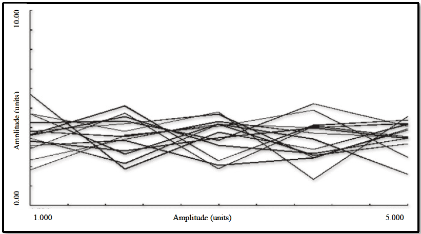
Figure description:
| Amplitude (units) | Series 1 | Series 2 | Series 3 | Series 4 | Series 5 | Series 6 | Series 7 | Series 8 | Series 9 | Series 10 |
|---|---|---|---|---|---|---|---|---|---|---|
| 1.000 | 4.8 | 4.3 | 4.1 | 3.9 | 3.7 | 3.5 | 3.4 | 3.1 | 2.8 | 2.5 |
| 2.000 | 2.8 | 3.8 | 4.8 | 4.2 | 3.4 | 4.0 | 3.6 | 2.6 | 3.2 | 3.0 |
| 3.000 | 4.2 | 4.4 | 3.2 | 3.6 | 4.2 | 2.6 | 4.0 | 3.4 | 2.8 | 3.8 |
| 4.000 | 3.6 | 3.4 | 5.0 | 4.2 | 3.8 | 4.0 | 2.2 | 3.2 | 3.4 | 2.8 |
| 5.000 | 3.4 | 4.2 | 3.2 | 4.4 | 3.6 | 3.8 | 3.6 | 4.0 | 2.8 | 2.4 |
Notes: The data values for the 10 estimated series are derived from visual inspection of the chart. Both axes are labeled 'Amplitude (units', though the Y-axis contains a typo ('Amnlitude'. The data points are captured at regular intervals corresponding to the tick marks on the X-axis from 1.000 to 5.000.))
Figure 516.8C-1. Input test data set.
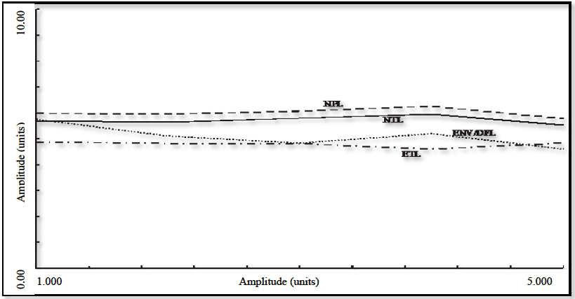
Figure description:
Legend
- NPL — color: black; symbol: Dashed line
- NIL — color: black; symbol: Solid line
- ENV/DFL — color: black; symbol: Dotted line
- ETL — color: black; symbol: Dash-dot line
| Amplitude (units) | NPL | NIL | ENV/DFL | ETL |
|---|---|---|---|---|
| 1.000 | 5.1 | 4.7 | 4.8 | 3.9 |
| 1.500 | 5.1 | 4.6 | 4.4 | 3.9 |
| 2.000 | 5.1 | 4.6 | 4.2 | 3.8 |
| 2.500 | 5.2 | 4.7 | 4.1 | 3.8 |
| 3.000 | 5.3 | 4.8 | 3.9 | 3.9 |
| 3.500 | 5.4 | 4.9 | 4.1 | 3.7 |
| 4.000 | 5.5 | 5.0 | 4.3 | 3.6 |
| 4.500 | 5.3 | 4.8 | 3.9 | 3.8 |
| 5.000 | 5.1 | 4.6 | 3.7 | 3.8 |
Notes: The x-axis and y-axis are both labeled 'Amplitude (units'. The y-axis ranges from 0.00 to 10.00. The x-axis ranges from 1.000 to 5.000 with tick marks every 0.5 units.)
Figure 516.8C-2. Parametric and non-parametric upper limits.
MIL-STD-810H METHOD
3.3 Post-Test
The following information shall be included in the test report.
- a. General. Information listed in Part One, paragraph. 5.13 of this Standard; and in Part One, Annex A, Task 406.
- b. Specific to this Method.
- (1) Duration of each exposure and number of exposures.
- (2) Status of the test item after each visual examination.
- (3) All response time histories and the information processed from these time histories. In general, under- processed information, the absolute acceleration maximax SRS, and the pseudo-velocity SRS should be supplied as a function of single degree-of-freedom oscillator undamped natural frequency. In certain cases, the ESD and FS may be supplied.
- (4) Test item and/or fixture modal analysis data and, if available, a mounted item/fixture modal analysis.
- (5) Any deviation from the test plan or default severities (e.g., drop surface).
516.8-3.3 Shock Velocity/Displacement Validation Criteria
Two steps are necessary for examining an unprocessed acceleration time history for purposes of validation.
- a. The first step is to clearly define the bandwidth of the measurement time history. The signal conditioning configuration and the ESD estimate to be discussed in paragraph 3.4 (below) will be helpful. The time history bandwidth will determine if TWR is a laboratory test option.
- b. The second step relates to integration of the time history to see if the velocity and displacement make physical sense. Velocity can usually be determined from direct integration of the shock acceleration after the shock has had its mean removed (velocity begins at zero and ends at zero), or has been high pass filtered to remove any DC component and other very low frequency information. Subsequent removal of the velocity mean or DC information in the velocity allows integration of the velocity to get displacement. As a minimum requirement, shock acceleration time traces should be integrated to provide velocity, and the velocity should have a clear physical interpretation, e.g., oscillatory behavior and near zero velocity at the "beginning" and the "end" of the shock. Velocity tends to be quite sensitive to sensor or signal conditioning anomalies that invalidate measurements. Integration of the velocity to obtain displacement should be considered an extended requirement, and reasonable values for displacement should be apparent. The form of velocity (or displacement) with respect to oscillatory behavior needs to be examined for reasonableness. That is, a form of velocity that displays little oscillatory behavior should be suspect. Figure 516.8B-4 displays velocity computed via mean removal alone. Figure 516.8B-5 displays the results of integrating velocity to arrive at displacement. For displacement, "DC" removal was performed on the velocity time history. Examination of both these plots, knowing the physical nature of the test, shows (1) reasonableness of peak amplitudes, and range from positive to negative values, (2) distinct and substantial oscillatory behavior during the "shock," and (3) characteristic pre- and post- shock noise floor behavior. It would appear that the bandlimited measurement does not have readily identifiable anomalies, and the acceleration time trace can be considered valid for further processing that is designed to either support or refute this validation.
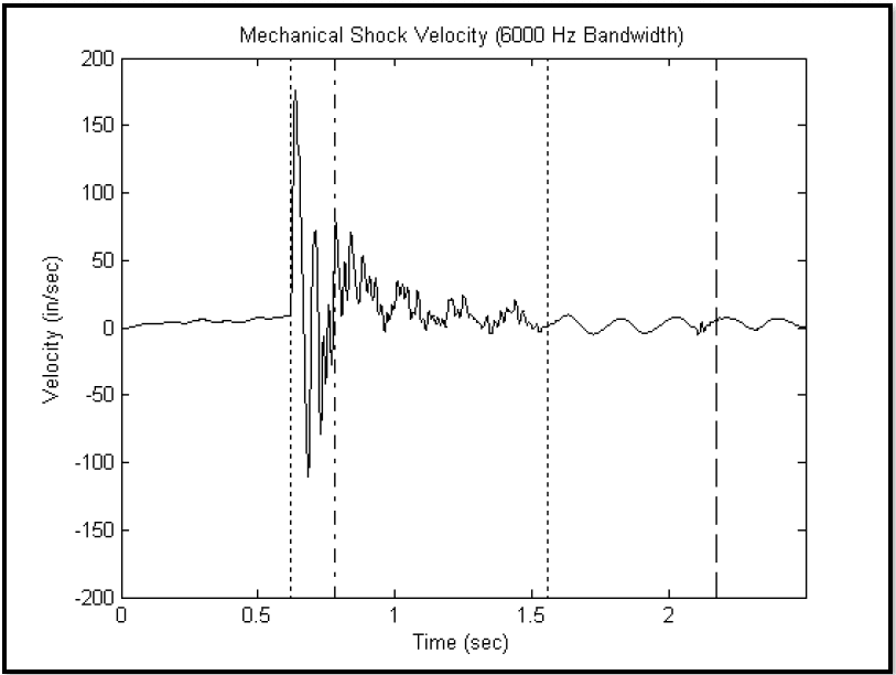
Figure description:
Mechanical Shock Velocity (6000 Hz Bandwidth
Mechanical Shock Velocity (6000 Hz Bandwidth
Annotations
- Start of shock (vertical_line - position: Time (sec ≈ 0.62))
- Boundary 1 (vertical_line - position: Time (sec ≈ 0.78))
- End of shock (vertical_line - position: Time (sec ≈ 1.55))
- Boundary 2 (vertical_line - position: Time (sec ≈ 2.18))
| Time (sec) | Velocity (in/sec) |
|---|---|
| 0.00 | 0.0 |
| 0.10 | 2.5 |
| 0.20 | 3.5 |
| 0.30 | 5.0 |
| 0.40 | 6.0 |
| 0.50 | 8.0 |
| 0.60 | 10.0 |
| 0.62 | 15.0 |
| 0.63 | 175.0 |
| 0.65 | 130.0 |
| 0.68 | -110.0 |
| 0.70 | -20.0 |
| 0.71 | 72.0 |
| 0.73 | -80.0 |
| 0.75 | 10.0 |
| 0.78 | 88.0 |
| 0.80 | 15.0 |
| 0.82 | -25.0 |
| 0.85 | 70.0 |
| 0.90 | 25.0 |
| 1.00 | 20.0 |
| 1.10 | 12.0 |
| 1.20 | 5.0 |
| 1.30 | 18.0 |
| 1.40 | 20.0 |
| 1.50 | 5.0 |
| 1.55 | 0.0 |
| 1.70 | -5.0 |
| 1.85 | 10.0 |
| 2.00 | -4.0 |
| 2.18 | 8.0 |
| 2.30 | -1.0 |
| 2.45 | 1.0 |
Notes: The chart shows a velocity time-history with a significant shock event occurring between approximately 0.62 and 1.55 seconds. Dotted and dashed vertical lines highlight specific phases of the shock and subsequent decay.
Figure 516.8B-4. Measurement velocity via integration of mean (DC) removed acceleration.
MIL-STD-810H
METHOD 516.8 ANNEX B
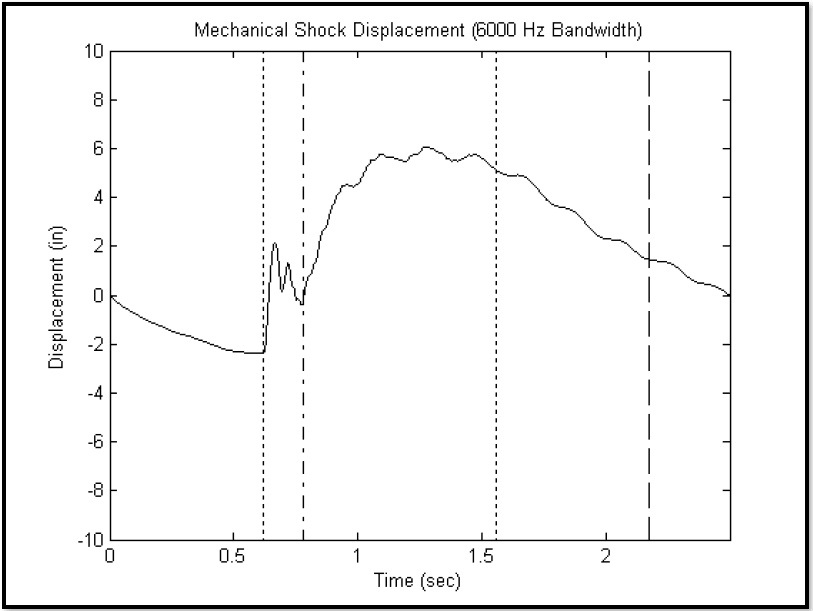
Figure description:
Mechanical Shock Displacement (6000 Hz Bandwidth
Mechanical Shock Displacement (6000 Hz Bandwidth
Annotations
- Event start marker (vertical_line - position: x ≈ 0.63)
- Transient transition marker (vertical_line - position: x ≈ 0.78)
- Decay start marker (vertical_line - position: x ≈ 1.56)
- Event end marker (vertical_line - position: x ≈ 2.18)
| Time (sec) | Displacement (in) |
|---|---|
| 0.00 | 0.00 |
| 0.10 | -0.60 |
| 0.20 | -1.10 |
| 0.30 | -1.60 |
| 0.40 | -2.00 |
| 0.50 | -2.30 |
| 0.60 | -2.35 |
| 0.63 | -2.35 |
| 0.64 | 1.80 |
| 0.68 | 2.10 |
| 0.70 | 0.20 |
| 0.72 | 1.30 |
| 0.74 | 0.20 |
| 0.76 | -0.20 |
| 0.78 | 0.20 |
| 0.85 | 1.80 |
| 0.90 | 3.50 |
| 1.00 | 5.20 |
| 1.10 | 5.70 |
| 1.20 | 5.50 |
| 1.30 | 6.00 |
| 1.40 | 5.50 |
| 1.50 | 5.80 |
| 1.56 | 5.10 |
| 1.60 | 4.80 |
| 1.70 | 4.80 |
| 1.80 | 3.80 |
| 1.90 | 3.50 |
| 2.00 | 2.40 |
| 2.10 | 2.20 |
| 2.18 | 1.40 |
| 2.30 | 0.80 |
| 2.40 | 0.40 |
| 2.50 | 0.00 |
Notes: The data values for Displacement were estimated from the plot line based on the provided axes. The vertical markers denote specific phases of the mechanical shock event.
Figure 516.8B-5. Measurement displacement via integration of velocity after mean (DC) removal.
At this point in the analysis, if the velocity and displacement validation checks, particularly the velocity validation check, do not seem to correspond with the physics of the test, a detailed investigation of the reason for this discrepancy must be instigated. For example, velocities that are not physically realizable call for such an investigation. For one of a kind and expensive tests, it may be possible to recover meaningful data based upon advanced processing techniques.
516.8-3.3 Non-parametric Upper Limits
The envelope limit (ENV) along with the upper distribution-free tolerance limit (DFL) for β proportion of the population set at 0.95 and γ confidence coefficient of 0.51 for N=14 samples is displayed in Figure 516.8C-2. This represents one curve with two interpretations. The 95 percent upper empirical tolerance limit (ETL) is also displayed on Figure 516.8C-2 where at least 95 percent of the values will be exceeded by this limit with 50 percent confidence. The data are displayed on Figure 516.8C-2 for comparison purposes.
3.4 ESD Estimate
The ESD is a single block periodiogram sampled at a uniform set of frequencies distributed over the bandwidth of interest, and displayed as a two-dimensional plot of amplitude units ("units² - sec/Hz") versus frequency in Hz. In determining the estimate, the Fast Fourier Transform block size must include the entire shock above the measurement system noise floor, interval T, otherwise the low frequency components will be biased. Selection of an analysis filter bandwidth may require padding with zeros beyond the effective duration, T. Zero padding results in a frequency interpolation of the ESD estimate. Generally, a rectangular window will be assumed in the time domain, however, other windows are permissible, e.g., Kaiser, as long as the analyst understands the effects of the window shape in the frequency domain, since time domain multiplication results in frequency domain convolution. The ESD description is useful for comparing the distribution of energy within selected frequency bands among several shocks, provided the analysis frequency bandwidth is the same, and it is realized that the estimates have approximately 100% normalized random error. Figure 516.8B-6 displays the ESD estimate for the shock time history in Figure 516.8B-1. By either (1) averaging n adjacent ESD ordinates (keeping estimate bias a minimum), or (2) averaging n independent, but statistically equivalent ESD estimates, the percentage of normalized random error can be decreased by a factor of 1/√n. Frequency averaging for periodiogram estimates is well defined in reference 6.1j. ESD estimates for noise floor segments tend not to be particularly useful for examining the validity of the measurement system because of the nondescript behavior of the noise floor.
MIL-STD-810H METHOD
516.8-3.4 Observations
The “flatness” of the upper limits on Figure 516.8C-2 attests to the homogeneity of the data in Table 516.8C-II. It is apparent from Figure 516.8C-2 that the upper limits for the parameters selected are not “statistically equivalent.” Of the two upper limit estimates, the NTL is favored if it can be established that the logarithm transform of the data set is approximately normally distributed. The closeness of the nonparametric envelopes attests also to the homogeneity of the data in Table 516.8C-II in addition to demonstrating, for this case at least, the non-statistical ENV, the statistically based DFL and the ETL basically agree with regard to the upper limit magnitude. For non-homogeneous data sets ETL would not be expected to agree with ENV or DFL. For small data sets, ETL may vary depending upon if parameter k rounds upward or downward.