519.8 GUNFIRE SHOCK CONTENTS
| Paragraph | Page | ||
|---|---|---|---|
| 1. | SCOPE | 1 | |
| 1.1 | PURPOSE | 1 | |
| 1.2 | APPLICATION | 1 | |
| 1.3 | LIMITATIONS. | 2 | |
| 2. | TAILORING GUIDANCE.. | 2 | |
| 2.1 | SELECTING THE GUNFIRE SHOCK METHOD. | 2 | |
| 2.1.1 | EFFECTS OF A GUNFIRE SHOCK ENVIRONMENT | 2 | |
| 2.1.2 | SEQUENCE AMONG OTHER METHODS. | 3 | |
| 2.2 | SELECTING A PROCEDURE.. | 4 | |
| 2.2.1 | PROCEDURE SELECTION CONSIDERATIONS. | 4 | |
| 2.2.2 | DIFFERENCE AMONG PROCEDURES. | 5 | |
| 2.3 | DETERMINE TEST LEVELS AND CONDITIONS | 6 | |
| 2.3.1 | GENERAL CONSIDERATIONS | 6 | |
| 2.3.2 | TEST CONDITIONS. | 6 | |
| 2.3.3 | TEST AXES AND NUMBER OF GUNFIRE SHOCK EVENTS.. | 6 | |
| 2.4 | TEST ITEM CONFIGURATION (SEE PART ONE, PARAGRAPH 5.8) | 7 | |
| 2.5 | CONTROLS | 7 | |
| 2.5.1 | CONTROL OPTIONS | 7 | |
| 2.5.1.1 | OPEN/CLOSED LOOP | 7 | |
| 2.5.1.2 | SINGLE POINT CONTROL | 7 | |
| 2.5.1.3 | MULTIPLE POINT CONTROL | 7 | |
| 2.5.2 | CONTROL METHODS | 7 | |
| 2.5.2.1 | WAVEFORM CONTROL | 7 | |
| 2.5.2.2 | SPECTRUM CONTROL. | 7 | |
| 3. | INFORMATION REQUIRED. | 8 | |
| 3.1 | PRETEST.. | 8 | |
| 3.2 | DURING TEST. | 9 | |
| 3.3 | POST-TEST | 9 | |
| 4. | TEST PROCESS | 10 | |
| 4.1 | TEST FACILITY | 10 | |
| 4.2 | CONTROLS | 10 | |
| 4.2.1 | MEASURED MATERIEL INPUT/RESPONSE TIME HISTORY UNDER TWR.. | 12 | |
| 4.2.2 | SRS GENERATED SHOCK TIME HISTORY PULSE SEQUENCE UNDER TWR. | 12 | |
| 4.2.3 | STOCHASTICALLY GENERATED MATERIEL INPUT FROM PRELIMINARY DESIGN SPECTRUM UNDER TWR | 12 | |
| 4.3 | TEST INTERRUPTION | 12 | |
| 4.3.1 | INTERRUPTION FROM FAILURE OR MALFUNCTION OF ASSOCIATED LABORATORY TEST EQUIPMENT | 13 | |
| 4.3.2 | INTERRUPTION DUE TO TEST ITEM OPERATION FAILURE | 13 | |
| 4.4 | TEST EXECUTION | 13 | |
| 4.4.1 | PREPARATION FOR TEST.. | 13 | |
MIL-STD-810H METHOD
519.8 CONTENTS - Continued
| Paragraph | Page |
|---|---|
| 4.4.1.1 PRETEST CHECKOUT | 13 |
| 4.4.1.2 PROCEDURE OVERVIEW | 13 |
| 4.4.1.3 TEST ITEM CONSIDERATIONS | 14 |
| 4.4.2 PROCEDURE I - MEASURED MATERIEL INPUT/RESPONSE TIME HISTORY UNDER TWR | 14 |
| 4.4.2.1 CONTROLS | 14 |
| 4.4.2.2 TEST TOLERANCES | 14 |
| 4.4.2.3 PROCEDURE STEPS | 14 |
| 4.4.2.4 ANALYSIS OF RESULTS | 14 |
| 4.4.3 PROCEDURE II - SRS GENERATED SHOCK TIME HISTORY PULSE SEQUENCE UNDER TWR | 15 |
| 4.4.3.1 CONTROLS | 15 |
| 4.4.3.2 TEST TOLERANCES | 15 |
| 4.4.3.3 PROCEDURE STEPS | 15 |
| 4.4.3.4 ANALYSIS OF RESULTS | 15 |
| 4.4.4 PROCEDURE III - STOCHASTICALLY GENERATED MATERIEL INPUT FROM PRELIMINARY DESIGN SPECTRUM | 15 |
| 4.4.4.1 CONTROLS | 15 |
| 5. ANALYSIS OF RESULTS | 16 |
| 6. REFERENCE/RELATED DOCUMENTS | 16 |
| 6.1 REFERENCED DOCUMENTS | 16 |
| 6.2 RELATED DOCUMENTS | 17 |
METHOD 519.8, ANNEX A GUIDELINES FOR PROCEDURE I - MEASURED MATERIEL INPUT/RESPONSE TIME HISTORY UNDER TWR
| 1. | SCOPE | A-1 |
| 1.1 | PURPOSE | .A-1 |
| 1.2 | APPLICATION | .A-1 |
| 2. | DEVELOPMENT | A-1 |
| 2.1 | BASIC CONSIDERATIONS FOR ENVIRONMENTAL DETERMINATION. | .A-1 |
| 2.2 | TEST CONFIGURATION | .A-1 |
| 2.3 | CREATING A DIGITAL FILE OF THE MEASURED GUNFIRE SHOCK INPUT TO THE MATERIEL | .A-2 |
| 2.4 | REPLICATING THE MEASURED GUNFIRE SHOCK MATERIEL INPUT IN LABORATORY TEST | .A-3 |
| 2.5 | POST-TEST PROCESSING | .A-4 |
| 2.6 | CONCLUSION. | .A-11 |
| 2.6.1 | GENERAL REMARKS. | .A-11 |
| 2.6.2 | STOCHASTIC GENERATION | .A-11 |
MIL-STD-810H METHOD
519.8 CONTENTS - Continued ANNEX A FIGURES
FIGURE 519.8A-1.
IN-SERVICE MEASURED GUNFIRE SHOCK: UNPROCESSED TIME TRACE (2000 RND/MIN AND
4000 RND/MIN
.A-2
FIGURE 519.8A-2.
UNPROCESSED TWR TEST REFERENCE, CONTROL, AND DIFFERENCE TIME TRACES (10 HZ TO
2000 Hz 25600 SPS).
..A-3
FIGURE 519.8A-3.
BANDLIMITED (10 HZ TO 2000 HZ) AND UNPROCESSED TWR TEST CONTROL TIME TRACES A-4
FIGURE 519.8A-4.
HIGH RESOLUTION REPRESENTATIVE MEMBERS FOR THE PULSE ENSEMBLES
(2000 ROUNDS/MINUTE).
..A-5
FIGURE 519.8A-5.
HIGH RESOLUTION REPRESENTATIVE MEMBERS FOR THE PULSE ENSEMBLES
(4000 ROUNDS/MINUTE).
A-6
FIGURE 519.8A-6.
STARMS DIFFERENCE BETWEEN CONTROL AND REFERENCE WITH CROSS-CORRELATION
ESTIMATE (DIFFERENCE: REF = 45.1 G-RMS / CROSS-CORRELATION).
A-7
FIGURE 519.8A-7.
STARMS FOR DIFFERENCE TIME TRACE(DIFFERENCE: REF = 45.1 G-RMS)
.A-8
FIGURE 519.8A-8.
QQ-PLOT FOR GAUSSIAN VERSUS DIFFERENCE TIME TRACE
.A-8
FIGURE 519.8A-9.
REFERENCE VERSUS CONTROL CROSS-PLOT
.A-9
FIGURE 519.8A-10a. PEAK STATISTIC DIFFERENCE...
.A-10
FIGURE 519.8A-10B. PEAK/VALLEY STATISTIC DIFFERENCE-QQ-PLOT.
.A-10
A TABLE
| TABLE 519.8A-I. | PEAK STATISTIC DIFFERENCE STATISTICS | A-11 |
|---|
METHOD 519.8, ANNEX B
GUIDELINES FOR PROCEDURE II - SRS GENERATED SHOCK TIME HISTORY PULSE SEQUENCE UNDER TWR
| 1. | SCOPE | B-1 |
|---|---|---|
| 1.1 | PURPOSE | B-1 |
| 1.2 | APPLICATION | B-1 |
| 2. | BASIC CONSIDERATIONS FOR DETERMINISTIC GENERATION OF A TIME TRACE HISTORY FROM A SRS ESTIMATE. | B-2 |
| 2.1 | INTRODUCTION | B-2 |
| 2.2 | SINGLE GUNFIRE SHOCK EVENT WITH SRS SPECIFICATION. | B-2 |
| 2.3 | MULTIPLE GUNFIRE SHOCK EVENTS WITH SRS CONSIDERATIONS | B-6 |
| 3. | CONCLUSION.. | B-6 |
B FIGURES
| FIGURE 519.8B-1. | GENERIC EXAMPLE GUNFIRE SRS REFERENCE | B-2 |
| FIGURE 519.8B-2. | DETERMINISTIC SRS SINE-BEAT SYNTHESIZED PULSE (EXTENDED OVER 20 MILLISECONDS FOR 50 HZ GUNFIRING RATE) | B-3 |
| FIGURE 519.8B-3. | CONCATENATED HIGH FREQUENCY SYNTHESIS (200-2000 Hz) | B-4 |
| FIGURE 519.8B-4. | BANDLIMITED RANDOM SYNTHESIS (10 Hz- 200 Hz). | B-5 |
| FIGURE 519.8B-5. | SYNTHESIZED ONE-SECOND GUNFIRE SHOCK PULSE TRAIN REFERENCE PER ADDITIVE MODEL | B-6 |
MIL-STD-810H
METHOD 519.8
CONTENTS - Continued METHOD 519.8, ANNEX C
METHOD 3318, ANNEX C GUIDELINES FOR PROCEDURE III - Stochastically generated Materiel Input from Preliminary
| 1. | SCOPE | C-1 |
| PART 1 –SPECTRUM PREDICTION METHODOLOGY FOR PRELIMINARY MATERIEL DESIGN | ||
| 1. | SCOPE | C-2 |
| 1.1 | PURPOSE | C-2 |
| 1.2 | APPLICATION | C-2 |
| 1.3 | LIMITATIONS. | C-2 |
| 2. | DEVELOPMENT. | C-2 |
| 2.1 | INTRODUCTION | C-2 |
| 2.2 | PREDICTING GUNFIRE VIBRATION SPECTRA | C-3 |
| 2.3 | DURATION OF TEST | C-10 |
| 2.4 | SPECTRUM GENERATION TECHNIQUES | C-10 |
| PART 2 - IMPLEMENTATION OF PREDICTED SPECTRUM METHODOLOGY FOR PRELIMINARY MATERIEL DESIGN | ||
| 1. | SCOPE | .C-11 |
| 1.1 | PURPOSE | .C-11 |
| 1.2 | TIME DOMAIN WINDOWED PULSE (TDWP). | .C-11 |
| 1.2.1 | INTRODUCTION | .C-11 |
| 1.2.2 | OUTLINE OF IMPLEMENTATION | .C-11 |
| 1.3 | RANDOM MODULATED HARMONIC PULSE (RMHP) | .C-12 |
| 1.3.1 | INTRODUCTION | .C-12 |
| 1.3.2 | OUTLINE OF IMPLEMENTATION | .C-12 |
| 2. | RECOMMENDED PROCEDURES. | .C-12 |
| 2.1 | RECOMMENDED PROCEDURE | C-12 |
| 2.2 | UNCERTAINTY FACTORS | .C-12 |
| 2.2.1 | SOR PREDICTION METHODOLOGY UNCERTAINTY. | C-12 |
| 2.2.2 | STOCHASTIC TWR GENERATION UNCERTAINTY | .C-13 |
| ANNEX C FIGURES | ||
| FIGURE 519.8C-1. | GENERALIZED GUNFIRE INDUCED VIBRATION SPECTRUM SHAPE | C-3 |
| FIGURE 519.8C-2. | THE DISTANCE PARAMETER (D) AND DEPTH PARAMETER (RS).. | .C-6 |
| FIGURE 519.8C-3. | MULTIPLE GUNS, CLOSELY GROUPED | .C-6 |
| FIGURE 519.8C-4. | TEST LEVEL REDUCTION DUE TO GUN STANDOFF PARAMETER. | C-7 |
| FIGURE 519.8C-5. | TEST LEVEL REDUCTION DUE TO MATERIEL MASS LOADING | C-7 |
| FIGURE 519.8C-6. | TEST LEVEL REDUCTION DUE TO DEPTH PARAMETER | C-8 |
| FIGURE 519.8C-7. | DECREASE IN VIBRATION LEVEL WITH VECTOR DISTANCE FROM GUN MUZZLE. | C-8 |
| FIGURE 519.8C-8. | GUNFIRE PEAK VIBRATION REDUCTION WITH DISTANCE | C-9 |
MIL-STD-810H METHOD
519.8 CONTENTS - Continued ANNEX C TABLES
| TABLE 519.8C-I. | SUGGESTED GENERALIZED PARAMETRIC EQUATIONS FOR GUNFIRE-INDUCED VIBRATION | C-4 |
| TABLE 519.8C-II. | TYPICAL GUN CONFIGURATIONS ASSOCIATED WITH AIRCRAFT CLASSES | C-5 |
| TABLE 519.8C-III. | GUN SPECIFICATIONS | C-5 |
Downloaded from https://www.everyspec.com
MIL-STD-810H METHOD 519.8
(This page is intentionally blank.)
MIL-STD-810H
METHOD 519.8
METHOD
519.8 GUNFIRE SHOCK
NOTE: Tailoring is essential. Select Methods, procedures, and parameter levels based on the tailoring process described in Part One, paragraph 4.2.2, and Annex C. Apply the general guidelines for laboratory test methods described in Part One, paragraph 5 of this Standard.
Due to extensive revision to this method, no change bars have been provided.
519.8 ANNEX A METHOD 519.8, ANNEX A
GUIDELINES FOR PROCEDURE I - MEASURED MATERIEL INPUT/RESPONSE TIME HISTORY UNDER TWR
519.8 ANNEX A
performed specifically for measurement data collection. The in-service test and laboratory replication included accelerometer measurement locations that were correlated.
519.8 ANNEX A
For the vendor software used in the TWR test, the phase relationship between the reference and control time traces is preserved (based upon a check of the cross-correlation function estimate between the control and reference time traces). Thus, one can proceed to compute the post-processed difference time trace by subtracting the reference time trace from the control time trace. Figure 519.8A-4 displays in high resolution six arbitrarily selected pulses for the reference, control and difference time traces for the 2000 round/minute gunfire rate. Figure 519.8A-5 provides the same information for the 4000 round/minute gunfire rate. In these two figures, even though the difference time trace scale is ten percent of the reference/control time scale, the difference time trace is generally not of a Gaussian form, and has generally large values correlated with peaks in the reference time trace.
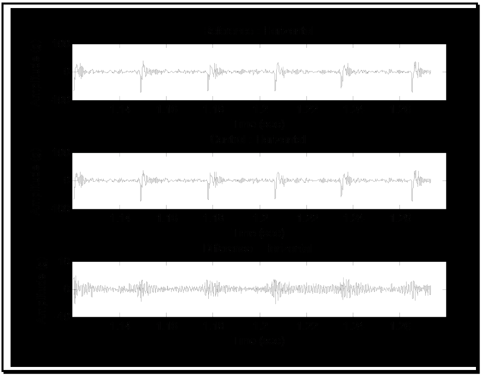
Figure description:
Horizontal Amplitude Comparison
Reference - Horizontal
| Time (sec) | Amplitude (g) |
|---|---|
| 1.125 | 15.0 |
| 1.127 | -82.0 |
| 1.129 | 25.0 |
| 1.135 | 5.0 |
| 1.145 | 10.0 |
| 1.148 | -78.0 |
| 1.150 | 35.0 |
| 1.160 | 0.0 |
| 1.170 | -5.0 |
| 1.175 | 15.0 |
| 1.178 | -80.0 |
| 1.180 | 28.0 |
| 1.190 | 2.0 |
| 1.200 | -5.0 |
| 1.204 | 20.0 |
| 1.206 | -75.0 |
| 1.208 | 32.0 |
| 1.220 | 0.0 |
| 1.233 | 25.0 |
| 1.235 | -60.0 |
| 1.237 | 20.0 |
| 1.245 | -5.0 |
| 1.263 | 38.0 |
| 1.265 | -72.0 |
| 1.267 | 22.0 |
| 1.275 | -5.0 |
Control - Horizontal
| Time (sec) | Amplitude (g) |
|---|---|
| 1.125 | 12.0 |
| 1.127 | -85.0 |
| 1.129 | 22.0 |
| 1.135 | 8.0 |
| 1.145 | 12.0 |
| 1.148 | -80.0 |
| 1.150 | 32.0 |
| 1.160 | 2.0 |
| 1.170 | -2.0 |
| 1.175 | 18.0 |
| 1.178 | -82.0 |
| 1.180 | 25.0 |
| 1.190 | 5.0 |
| 1.200 | -2.0 |
| 1.204 | 22.0 |
| 1.206 | -78.0 |
| 1.208 | 30.0 |
| 1.220 | 3.0 |
| 1.233 | 28.0 |
| 1.235 | -65.0 |
| 1.237 | 18.0 |
| 1.245 | -2.0 |
| 1.263 | 35.0 |
| 1.265 | -75.0 |
| 1.267 | 20.0 |
| 1.275 | -2.0 |
Difference - Horizontal
| Time (sec) | Amplitude (g) |
|---|---|
| 1.125 | 3.0 |
| 1.130 | -3.0 |
| 1.140 | 1.0 |
| 1.150 | -4.0 |
| 1.160 | 2.0 |
| 1.170 | -2.5 |
| 1.180 | 3.5 |
| 1.190 | -1.0 |
| 1.200 | 2.0 |
| 1.210 | -4.5 |
| 1.220 | 4.0 |
| 1.230 | -2.0 |
| 1.240 | 3.0 |
| 1.250 | -3.5 |
| 1.260 | 2.5 |
| 1.270 | -4.0 |
| 1.275 | 1.5 |
Notes: The plots show time-series signals in the horizontal direction. The 'Reference' and 'Control' signals are very similar, characterized by high-frequency noise and periodic high-magnitude negative spikes reaching approximately -80g. The 'Difference' plot shows the residual after subtracting Control from Reference, which is centered at zero with a significantly lower amplitude range (within +/- 5g.)
Figure 519.8A-4. High resolution representative members for the pulse ensembles (2000 rounds/minute).
MIL-STD-810H
METHOD 519.8 ANNEX A
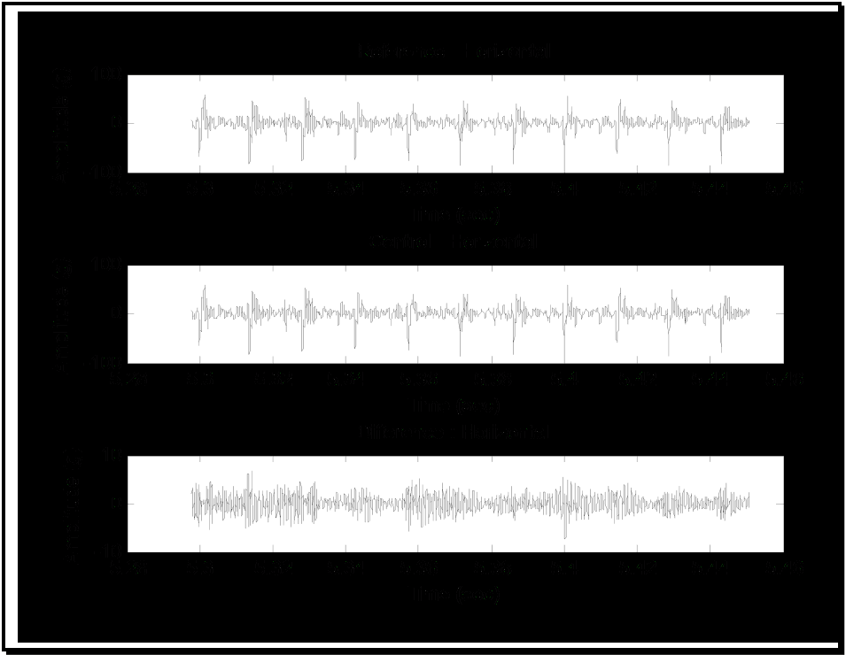
Figure description:
Reference - Horizontal
| Time (sec) | Amplitude (g) |
|---|---|
| 5.295 | 0 |
| 5.302 | 58 |
| 5.308 | -35 |
| 5.315 | 45 |
| 5.321 | -38 |
| 5.328 | 55 |
| 5.335 | -42 |
| 5.342 | 50 |
| 5.348 | -32 |
| 5.356 | 38 |
| 5.362 | -28 |
| 5.372 | 35 |
| 5.378 | -22 |
| 5.385 | 42 |
| 5.392 | -30 |
| 5.401 | 52 |
| 5.408 | -38 |
| 5.415 | 50 |
| 5.422 | -45 |
| 5.430 | 46 |
| 5.437 | -35 |
| 5.443 | 36 |
| 5.450 | -22 |
Control - Horizontal
| Time (sec) | Amplitude (g) |
|---|---|
| 5.295 | 0 |
| 5.302 | 54 |
| 5.308 | -32 |
| 5.315 | 42 |
| 5.321 | -35 |
| 5.328 | 51 |
| 5.335 | -40 |
| 5.342 | 46 |
| 5.348 | -30 |
| 5.356 | 35 |
| 5.362 | -25 |
| 5.372 | 32 |
| 5.378 | -20 |
| 5.385 | 39 |
| 5.392 | -28 |
| 5.401 | 49 |
| 5.408 | -35 |
| 5.415 | 47 |
| 5.422 | -42 |
| 5.430 | 43 |
| 5.437 | -32 |
| 5.443 | 33 |
| 5.450 | -20 |
Difference - Horizontal
| Time (sec) | Amplitude (g) |
|---|---|
| 5.302 | 4 |
| 5.308 | -3 |
| 5.315 | 3 |
| 5.321 | -3 |
| 5.328 | 4 |
| 5.335 | -2 |
| 5.342 | 4 |
| 5.348 | -2 |
| 5.356 | 3 |
| 5.362 | -3 |
| 5.372 | 3 |
| 5.378 | -2 |
| 5.385 | 3 |
| 5.392 | -2 |
| 5.401 | 3 |
| 5.408 | -3 |
| 5.415 | 3 |
| 5.422 | -3 |
| 5.430 | 3 |
| 5.437 | -3 |
| 5.443 | 3 |
| 5.450 | -2 |
Notes: The figure contains three time-series plots representing acceleration data in g. The X-axis for all charts is 'Time (sec' ranging from 5.28 to 5.46. The Y-axis for the 'Reference' and 'Control' charts ranges from -100 to 100, while the 'Difference' chart is scaled from -10 to 10. Data points in the markdown tables are representative samples of the high-frequency oscillation shown in the image.)
Figure 519.8A-5. High resolution representative members for the pulse ensembles (4000 rounds/minute).
Method 525.2 provides basic guidance on test tolerance specification but, in general, Method 525.2 requires that test tolerance criteria be tailored according to the form of time trace that is being replicated. For the gunfire shock environment, test tolerances are most meaningfully established in the time domain for the entire time trace (for ensemble processing pulse ensemble time based statistics along with frequency domain ESD estimates for both gunfire rates would provide supplementary criteria).
For test tolerance assessment the following test tolerance criteria are established:
- a. Short-Time-Average-Root-Mean-Square (STARMS) of the control time trace and of the reference time trace, when differenced, be less in absolute value than 1.0 dB (approximately 12 percent) at 90 percent of the STARMS estimate points when the difference is referenced to the maximum STARMS for the reference time trace. The short-time averaging time is not to exceed 0.1 of the gunfire pulse period. In addition plot of the cross-correlation estimate between control and reference for STARMS, i.e., for rms levels, is to be within 0.90 at 90 percent of the STARMS estimate points. (This tolerance criterion relates to the rms estimate differences between the control and reference time traces - it tends to be quite broad.)
- b. STARMS applied to the difference time trace is to be less than -15 dB (approximately 1.8 percent) when referenced to the maximum STARMS reference time trace level at 90 percent of the STARMS estimate points. The short-time averaging time is not to exceed 0.1 of the gunfire pulse period. (This tolerance criterion in effect compares the "noise" as represented by the difference time trace to the "signal" as represented by maximum STARMS of the reference time trace.)
MIL-STD-810H METHOD
519.8 ANNEX A
- c. Ideally the difference time trace amplitudes are Gaussian distributed. Usually this is never the case. It is required that qq-plot magnitudes beyond Gaussian three-sigma positive and negative limits not exceed the following:
For positive (negative) long tail distribution greater than 1.0 dB (approximately +12 percent) when referenced to the maximum absolute reference time trace positive (negative) peak, and;
For positive (negative) short tail distribution less than - 1.0 dB (approximately - 11 percent) when referenced to the maximum absolute reference time trace positive (negative) peak.
These test tolerance criteria are designed to compare reference and control time traces based upon their perfect correlation in time. If there exists a phase difference between the time traces, then none of the above test tolerance criteria are valid. If these test tolerance criteria can be satisfied, the test performance will be established.
Figure 519.8A-6 displays STARMS level difference between control and reference time traces where the short-time averaging time was selected to be 0.1*60/4000 = 0.0015 seconds over the entire time trace, and the maximum reference rms level was 100 g-rms. For each of the short-time-average rms estimates, the cross-correlation estimate between reference and control was computed and displayed.
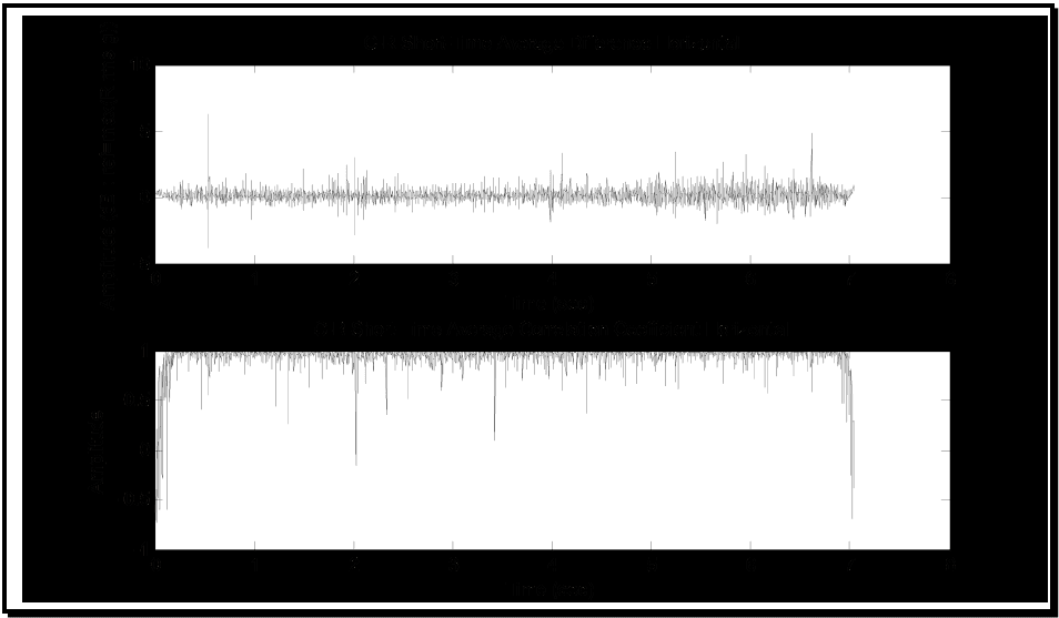
Figure description:
CIR Horizontal Analysis
CIR Short-Time Average Difference Horizontal
| Time (sec) | Amplitude (dB : ref=max(R rms)) |
|---|---|
| 0.0 | 0.3 |
| 0.2 | -0.5 |
| 0.5 | 6.2 |
| 0.5 | -3.8 |
| 1.0 | 0.1 |
| 1.5 | -0.4 |
| 1.8 | 2.8 |
| 2.0 | -2.5 |
| 2.3 | 1.5 |
| 2.8 | -0.2 |
| 3.2 | 0.8 |
| 3.8 | -1.2 |
| 4.1 | 3.4 |
| 4.5 | 0.2 |
| 5.0 | -0.7 |
| 5.4 | 3.5 |
| 5.8 | -1.8 |
| 6.2 | 2.4 |
| 6.6 | 4.9 |
| 7.0 | 0.5 |
CIR Short-Time Average Correlation Coefficient Horizontal
| Time (sec) | Amplitude |
|---|---|
| 0.0 | -0.65 |
| 0.1 | 0.90 |
| 0.3 | 0.98 |
| 0.5 | 0.42 |
| 0.8 | 0.95 |
| 1.2 | 0.99 |
| 1.6 | 0.92 |
| 1.9 | 0.15 |
| 2.0 | -0.18 |
| 2.2 | 0.38 |
| 2.6 | 0.96 |
| 3.1 | 0.97 |
| 3.5 | 0.12 |
| 4.0 | 0.94 |
| 4.6 | 0.98 |
| 5.2 | 0.90 |
| 5.7 | 0.82 |
| 6.1 | 0.58 |
| 6.5 | 0.91 |
| 6.9 | 0.96 |
| 7.0 | -0.75 |
Notes: The signals are plotted against a time axis from 0 to 8 seconds, though data series terminate at 7 seconds. The first plot shows amplitude in dB with a baseline around 0 and several sharp spikes. The second plot shows a correlation coefficient mostly near 1.0 with several significant downward drops.
Figure 519.8A-6. STARMS difference between control and reference with cross-correlation estimate. (Difference: ref = 45.1 g-rms /cross-correlation)
Figure 519.8A-7 displays STARMS for the difference time trace, where the short-time averaging time was selected to be 0.1*60/4000 = 0.0015 seconds over the entire time trace, and the maximum reference rms level was 45.1 g-rms.
MIL-STD-810H
METHOD 519.8 ANNEX A
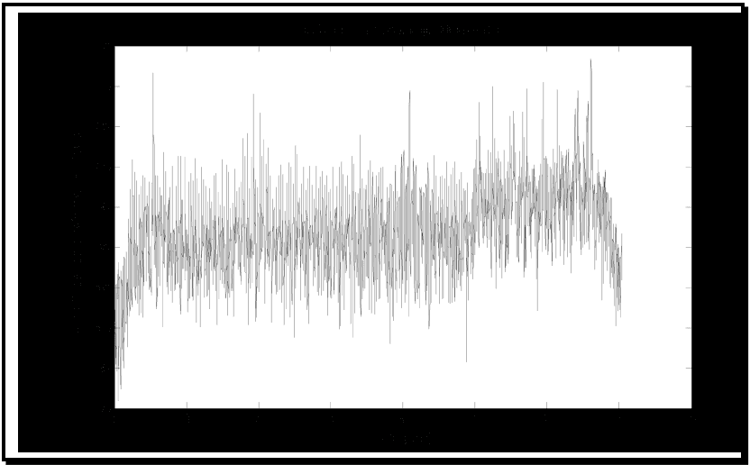
Figure description:
ID Short Time Average Horizontal
ID Short Time Average Horizontal
| Time (sec) | Amplitude (dB re: max (A rms g)) |
|---|---|
| 0.00 | -53.2 |
| 0.05 | -48.5 |
| 0.10 | -38.2 |
| 0.15 | -44.1 |
| 0.20 | -32.5 |
| 0.30 | -36.4 |
| 0.40 | -31.8 |
| 0.50 | -13.2 |
| 0.60 | -34.5 |
| 0.70 | -31.2 |
| 0.80 | -35.6 |
| 0.90 | -30.5 |
| 1.00 | -33.8 |
| 1.25 | -34.2 |
| 1.50 | -32.7 |
| 1.75 | -33.5 |
| 1.90 | -15.8 |
| 2.00 | -34.2 |
| 2.25 | -33.1 |
| 2.50 | -32.4 |
| 2.75 | -33.6 |
| 3.00 | -32.9 |
| 3.25 | -34.5 |
| 3.50 | -33.8 |
| 3.75 | -32.2 |
| 4.00 | -31.5 |
| 4.10 | -15.5 |
| 4.25 | -34.8 |
| 4.50 | -33.2 |
| 4.75 | -34.1 |
| 4.85 | -44.5 |
| 5.00 | -14.8 |
| 5.10 | -28.5 |
| 5.25 | -27.2 |
| 5.40 | -14.9 |
| 5.50 | -28.4 |
| 5.75 | -26.5 |
| 5.85 | -15.1 |
| 6.00 | -14.2 |
| 6.25 | -15.3 |
| 6.50 | -16.2 |
| 6.65 | -11.8 |
| 6.75 | -25.8 |
| 6.90 | -28.5 |
| 7.00 | -34.2 |
| 7.05 | -46.5 |
Notes: The data depicts a highly oscillatory signal. The provided table captures key milestones including the initial rise, baseline oscillations, major peaks, and the shift to a slightly higher average amplitude after 5 seconds, followed by the final drop-off around 7 seconds.
Figure 519.8A-7. STARMS for difference time trace. (Difference: ref = 45.1 g-rms)
The qq-plot for the difference time trace is displayed in Figure 519.8A-8, along with the three-sigma Gaussian limits. It is clear that the difference time trace is not Gaussian distributed, but has a long tail structure. This appears to be characteristic of most all TWR tests, and somewhat complicates tolerance specification. But for reference peak amplitudes on the order of 100g in the negative and positive directions, generally the maximum differences are within 1dB of the peak reference magnitudes.
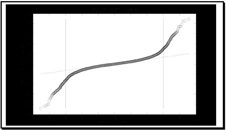
Figure description:
Difference qq-plot horizontal
Difference qq-plot horizontal
Annotations
- Left boundary line (vertical_line - position: x = -3)
- Right boundary line (vertical_line - position: x = 3)
- Linear reference line (text_label - position: y ≈ 1.25x)
| Normal Quantiles | Horizontal Amplitude (g) | Reference Line (Horizontal Amplitude (g)) |
|---|---|---|
| -4.51 | -22.1 | -5.64 |
| -4.25 | -21.2 | -5.31 |
| -4.13 | -20.5 | -5.16 |
| -4.02 | -18.3 | -5.03 |
| -3.75 | -15.5 | -4.69 |
| -3.50 | -13.9 | -4.38 |
| -3.25 | -12.2 | -4.06 |
| -3.00 | -10.0 | -3.75 |
| -2.75 | -8.2 | -3.44 |
| -2.50 | -6.6 | -3.13 |
| -2.25 | -5.5 | -2.81 |
| -2.00 | -4.5 | -2.50 |
| -1.75 | -3.8 | -2.19 |
| -1.50 | -3.2 | -1.88 |
| -1.25 | -2.7 | -1.56 |
| -1.00 | -2.2 | -1.25 |
| -0.75 | -1.7 | -0.94 |
| -0.50 | -1.2 | -0.63 |
| -0.25 | -0.7 | -0.31 |
| 0.00 | 0.0 | 0.00 |
| 0.25 | 0.5 | 0.31 |
| 0.50 | 1.0 | 0.63 |
| 0.75 | 1.5 | 0.94 |
| 1.00 | 2.0 | 1.25 |
| 1.25 | 2.5 | 1.56 |
| 1.50 | 3.0 | 1.88 |
| 1.75 | 3.6 | 2.19 |
| 2.00 | 4.3 | 2.50 |
| 2.25 | 5.3 | 2.81 |
| 2.50 | 6.4 | 3.13 |
| 2.75 | 8.0 | 3.44 |
| 3.00 | 9.9 | 3.75 |
| 3.25 | 12.1 | 4.06 |
| 3.50 | 14.1 | 4.38 |
| 3.75 | 16.0 | 4.69 |
| 4.02 | 18.4 | 5.03 |
| 4.25 | 21.1 | 5.31 |
| 4.55 | 22.3 | 5.69 |
Notes: The chart is a Q-Q plot comparing Horizontal Amplitude (g against Normal Quantiles. It indicates a distribution with significantly heavier tails than a standard normal distribution, as evidenced by the S-shaped deviation from the linear reference line. Vertical reference lines are indicated at quantiles of -3 and 3.)
Figure 519.8A-8. qq-plot for Gaussian versus difference time trace.
Figure 519.8A-9 displays cross-plot information for reference versus control time traces. It is unclear how this information can be used for establishing test tolerance. Simple confidence intervals around a straight line fit of the cross plot points is difficult to interpret, and is contrary to intuition. Typically such confidence intervals as a result of
MIL-STD-810H METHOD
519.8 ANNEX A
straight-line regression fits are a minimum distance apart for values near zero, and a maximum distance apart near the end points or peaks. For TWR testing, the larger differences or errors tend to be for values near zero where noise has a greater effect on the "signal" defined by the reference time trace.
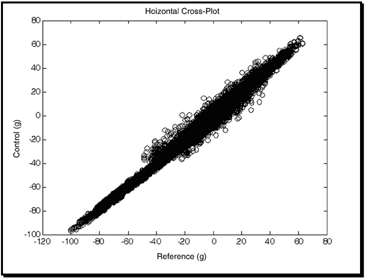
Figure description:
Hoizontal Cross-Plot
Hoizontal Cross-Plot
| Reference (g) | Control (g) |
|---|---|
| -101.3 | -96.5 |
| -98.2 | -94.1 |
| -89.5 | -87.8 |
| -80.4 | -78.2 |
| -70.1 | -68.5 |
| -60.8 | -59.3 |
| -50.2 | -48.1 |
| -48.5 | -35.4 |
| -45.1 | -42.8 |
| -40.6 | -28.2 |
| -38.4 | -37.5 |
| -32.1 | -15.4 |
| -30.5 | -34.8 |
| -25.6 | -22.1 |
| -20.2 | -2.1 |
| -19.8 | -32.4 |
| -15.4 | -18.7 |
| -10.1 | 12.5 |
| -8.5 | -20.3 |
| -1.2 | 15.6 |
| 0.5 | -12.4 |
| 5.4 | 22.1 |
| 8.2 | -8.5 |
| 15.6 | 32.4 |
| 18.2 | 4.5 |
| 25.4 | 45.1 |
| 28.1 | 8.2 |
| 35.6 | 48.7 |
| 38.4 | 25.1 |
| 45.2 | 55.4 |
| 48.1 | 42.1 |
| 55.6 | 62.4 |
| 60.2 | 58.1 |
| 62.8 | 65.7 |
Notes: The chart is a dense scatter plot showing a strong positive linear correlation between 'Reference (g' and 'Control (g'. The spread (variance of the 'Control' values relative to 'Reference' values increases significantly in the middle range, approximately between -45 and +40 on the x-axis, while being very tight at the negative extreme. The title contains a typo ('Hoizontal' instead of 'Horizontal' as seen in the original image.))))
Figure 519.8A-9. Reference versus control cross-plot.
Figure 519.8A-10 provides some initial information on the relationship between the reference and control peak structure. Detailed modeling of peak structure could be performed here, however, two basic considerations must be examined. First, an assumption that peak information is vital to the integrity of the test materiel must be established (peak time trace information is generally only loosely correlated with test materiel integrity - the pseudo-velocity shock response spectrum represents materiel stress better). Second, a decision must be made as to if the unprocessed (non-band limited) control time trace, or the processed (band limited) control time trace is to be compared with the reference time trace relative to peak information. Peak modeling and subsequent interpretation must consider both assumption and decision. In this Annex, a simple time trace plot along with a normal qq-plot is provided for the difference between a reference time trace peak (or valley), and the corresponding control time trace value (that may not represent a peak or valley response). Reference and control time traces have a common bandwidth. Statistics of this somewhat “stationary” appearing serial set of random variables (not a uniformly sampled time trace) are also provided in Table 519.8A-1.
MIL-STD-810H METHOD 519.8 ANNEX A
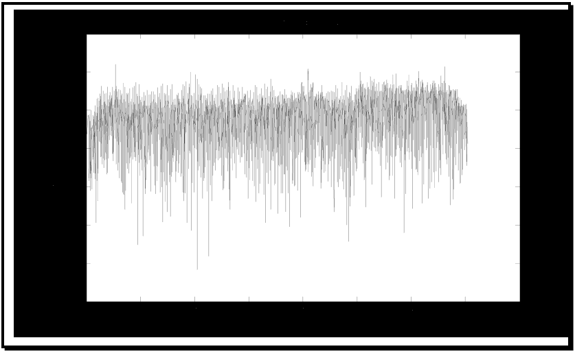
Figure description:
Peak Difference Horizontal
Peak Difference Horizontal
| Time (sec) | Amplitude (dB ref max(R)) |
|---|---|
| 0.0 | -75 |
| 0.2 | -45 |
| 0.5 | -15 |
| 0.8 | -60 |
| 1.0 | -55 |
| 1.5 | -50 |
| 2.0 | -123 |
| 2.2 | -115 |
| 2.5 | -50 |
| 3.0 | -45 |
| 3.5 | -40 |
| 4.1 | -20 |
| 4.5 | -55 |
| 5.0 | -108 |
| 5.5 | -35 |
| 5.8 | -104 |
| 6.2 | -22 |
| 6.5 | -30 |
| 7.0 | -68 |
Notes: The signal represents a high-frequency horizontal peak difference measured in dB over a 7-second period. The plot shows significant noise with extreme spikes and troughs ranging approximately between -15 dB and -125 dB.
Figure 519.8A-10a. Peak statistic difference.
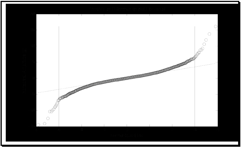
Figure description:
Peak/Valley Difference Analysis
Peak/Valley Difference qq-plot Horizontal
Annotations
- Negative Boundary (vertical_line - position: x = -3)
- Positive Boundary (vertical_line - position: x = 3)
- Theoretical Distribution Line (text_label - position: y ≈ 1.15x)
| Normal Quantiles | Horizontal Amplitude (g) | Theoretical Reference Line |
|---|---|---|
| -3.9 | -14.3 | -4.49 |
| -3.6 | -14.1 | -4.14 |
| -3.5 | -12.4 | -4.03 |
| -3.4 | -10.3 | -3.91 |
| -3.3 | -9.9 | -3.80 |
| -3.2 | -8.7 | -3.68 |
| -3.1 | -7.5 | -3.57 |
| -3.0 | -6.4 | -3.45 |
| -2.8 | -5.8 | -3.22 |
| -2.6 | -5.3 | -2.99 |
| -2.4 | -4.6 | -2.76 |
| -2.2 | -4.1 | -2.53 |
| -2.0 | -3.5 | -2.30 |
| -1.8 | -3.1 | -2.07 |
| -1.6 | -2.7 | -1.84 |
| -1.4 | -2.3 | -1.61 |
| -1.2 | -1.9 | -1.38 |
| -1.0 | -1.6 | -1.15 |
| -0.8 | -1.2 | -0.92 |
| -0.6 | -0.9 | -0.69 |
| -0.4 | -0.6 | -0.46 |
| -0.2 | -0.3 | -0.23 |
| 0.0 | 0.0 | 0.00 |
| 0.2 | 0.3 | 0.23 |
| 0.4 | 0.6 | 0.46 |
| 0.6 | 1.0 | 0.69 |
| 0.8 | 1.3 | 0.92 |
| 1.0 | 1.7 | 1.15 |
| 1.2 | 2.0 | 1.38 |
| 1.4 | 2.4 | 1.61 |
| 1.6 | 2.9 | 1.84 |
| 1.8 | 3.4 | 2.07 |
| 2.0 | 3.9 | 2.30 |
| 2.2 | 4.4 | 2.53 |
| 2.4 | 4.8 | 2.76 |
| 2.6 | 5.3 | 2.99 |
| 2.8 | 5.8 | 3.22 |
| 3.0 | 6.4 | 3.45 |
| 3.1 | 7.1 | 3.57 |
| 3.2 | 7.8 | 3.68 |
| 3.3 | 8.6 | 3.80 |
| 3.4 | 9.3 | 3.91 |
| 3.5 | 10.5 | 4.03 |
| 3.6 | 11.8 | 4.14 |
| 3.7 | 13.7 | 4.26 |
| 3.9 | 16.1 | 4.49 |
Notes: The data points represent the horizontal amplitude of peak/valley differences plotted against normal quantiles. The S-shaped deviation from the reference line indicates that the distribution has heavier tails than a normal distribution.
Figure 519.8A-10b. Peak/valley statistic difference - qq-plot.
MIL-STD-810H
METHOD 519.8 ANNEX A
The minimum, maximum, mean, standard deviation, skewness, and kurtosis of the peak statistic difference serial time sample is provided in the Table 519.8A-I.
| Minimum peak difference | -14.48 |
| Maximum peak difference | 16.14 |
| Mean peak difference | 0.07 |
| Root-Mean-Square peak difference | 1.53 |
| Skewness for peak difference | -0.06 |
| Kurtosis for peak difference | 10.17 |
519.8 ANNEX B
frequencies below the gunfire rate based upon the proposed test length (in terms of number of pulses at the gunfiring rate) can only be accounted for in an ad hoc manner.
519.8 ANNEX B Figure 519.8B-1. Generic example gunfire SRS reference
Figure 519.8B-2 displays a single deterministic pulse that has been generated from the Method 516.8 SRS algorithm implemented via the “sine-beat” procedure over 0.02 seconds (the period of the gunfire). Due to the short duration associated with the period of an individual frequency component, the low frequency limit in the synthesis is recommended to be one to two octaves above the gunfire frequency. This will allow inclusion of a reasonable number of cycles of the lower frequency components in the synthesis process. The resulting synthesis illustrated in Figure 519.8-B-2 was based on the reference SRS of Figure 519.8B-1 between 200 and 2000 Hz. It is noted that valid SRS information existing below the low frequency limit (200 Hz in this example) has been suppressed in the analytically generated pulse. The low SRS natural frequencies are artifacts of the variations between individual pulses in the original multiple shot measured time history. The low frequency information will be synthesized in a subsequent step.
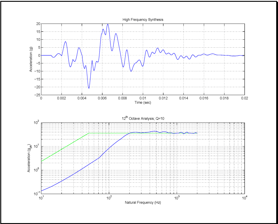
Figure description:
High Frequency Synthesis
| Time (sec) | Acceleration (g) |
|---|---|
| 0.000 | 0.0 |
| 0.001 | 0.0 |
| 0.0015 | -1.0 |
| 0.002 | 0.0 |
| 0.0024 | 8.5 |
| 0.0028 | -2.0 |
| 0.003 | -7.5 |
| 0.0034 | -3.0 |
| 0.0038 | 5.0 |
| 0.0042 | -5.0 |
| 0.0044 | -8.0 |
| 0.0047 | -21.0 |
| 0.005 | -3.5 |
| 0.0052 | -10.0 |
| 0.0054 | -4.0 |
| 0.006 | 13.0 |
| 0.0062 | 16.5 |
| 0.0065 | 19.5 |
| 0.007 | 3.0 |
| 0.0074 | 14.0 |
| 0.0078 | 5.0 |
| 0.008 | -3.5 |
| 0.0082 | -8.0 |
| 0.0085 | 3.5 |
| 0.0088 | -10.0 |
| 0.0095 | -3.0 |
| 0.010 | -7.0 |
| 0.0105 | 3.5 |
| 0.011 | -1.0 |
| 0.0115 | 4.5 |
| 0.012 | 1.5 |
| 0.0125 | 3.5 |
| 0.013 | 0.5 |
| 0.0135 | 1.0 |
| 0.014 | -1.5 |
| 0.0145 | 0.0 |
| 0.015 | -2.5 |
| 0.016 | 0.5 |
| 0.017 | 1.0 |
| 0.018 | 0.2 |
| 0.019 | -0.5 |
| 0.020 | 0.0 |
12th Octave Analysis; Q=10
| Natural Frequency (Hz) | Blue Series (g_pk) | Green Series (g_pk) |
|---|---|---|
| 10 | 0.12 | 2.3 |
| 20 | 0.35 | 7.0 |
| 30 | 0.70 | 14.0 |
| 40 | 1.10 | 25.0 |
| 50 | 1.70 | 35.0 |
| 60 | 2.50 | 35.0 |
| 70 | 3.50 | 35.0 |
| 100 | 10.0 | 35.0 |
| 150 | 25.0 | 35.0 |
| 200 | 35.0 | 35.0 |
| 300 | 40.0 | 35.0 |
| 400 | 43.0 | 35.0 |
| 500 | 45.0 | 35.0 |
| 600 | 40.0 | 35.0 |
| 700 | 42.0 | 35.0 |
| 800 | 38.0 | 35.0 |
| 1000 | 36.0 | 35.0 |
| 1200 | 41.0 | 35.0 |
| 1400 | 35.0 | 35.0 |
| 1600 | 41.0 | 35.0 |
| 2000 | 35.0 | 35.0 |
Notes: The second chart uses logarithmic scales for both axes.
Figure 519.8B-2. Deterministic SRS sine-beat synthesized pulse (extended over 20 milliseconds for 50 Hz gunfiring rate).
Figure 519.8B-3 displays the concatenated pulse to the specified duration (1 second bursts for this example). This concatenated pulse representing the “gunfire event” provides an SRS estimate as compared to the specified SRS. The prescribed duration of the concatenation will artificially introduce some low natural frequency SRS information but usually not enough information such that the SRS tolerance in Method 516.8 will be met. Guidance on addressing the low frequency portion of the SRS follows.
MIL-STD-810H
METHOD 519.8 ANNEX B
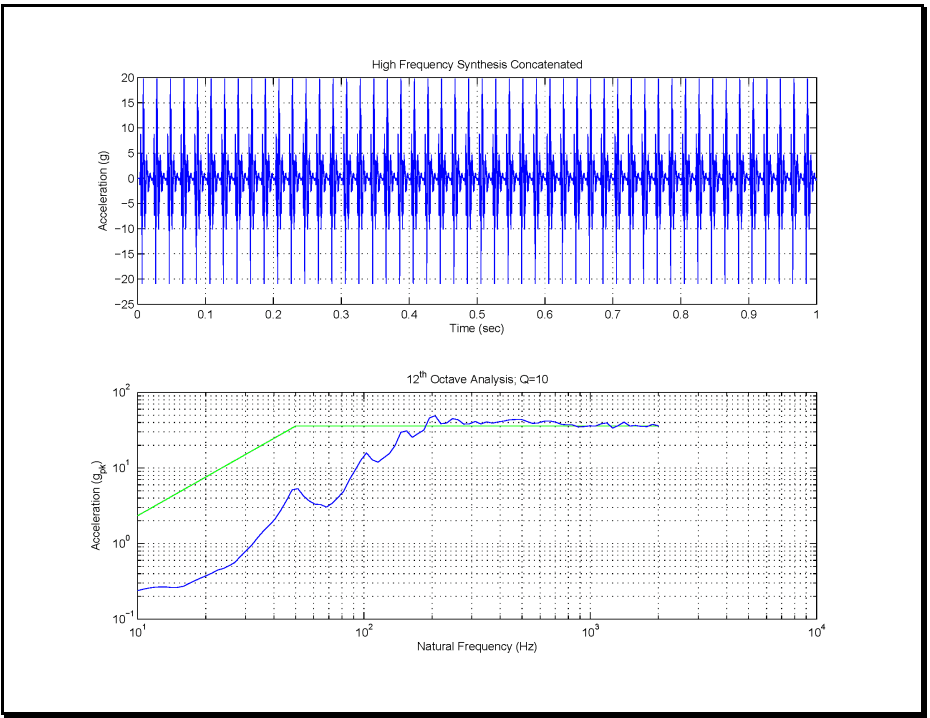
Figure description:
Shock Response and Spectral Analysis
High Frequency Synthesis Concatenated
| Time (sec) | Acceleration (g) |
|---|---|
| 0.00 | 0.0 |
| 0.01 | 20.0 |
| 0.02 | -21.0 |
| 0.03 | 20.0 |
| 0.04 | -21.0 |
| 0.05 | 20.0 |
| 0.06 | -21.0 |
| 0.07 | 20.0 |
| 0.08 | -21.0 |
| 0.09 | 20.0 |
| 0.10 | -21.0 |
| 0.20 | -21.0 |
| 0.30 | -21.0 |
| 0.40 | -21.0 |
| 0.50 | -21.0 |
| 0.60 | -21.0 |
| 0.70 | -21.0 |
| 0.80 | -21.0 |
| 0.90 | -21.0 |
| 1.00 | -21.0 |
12th Octave Analysis; Q=10
Legend
- Analysis curve — color: blue; symbol: Solid line
- Reference/Limit curve — color: green; symbol: Solid line
| Natural Frequency (Hz) | Blue Curve (g_pk) | Green Curve (g_pk) |
|---|---|---|
| 10 | 0.25 | 2.5 |
| 20 | 0.45 | 10.0 |
| 30 | 0.8 | 20.0 |
| 40 | 2.5 | 30.0 |
| 50 | 5.5 | 35.0 |
| 60 | 4.0 | 35.0 |
| 80 | 6.0 | 35.0 |
| 100 | 15.0 | 35.0 |
| 120 | 11.0 | 35.0 |
| 150 | 30.0 | 35.0 |
| 180 | 25.0 | 35.0 |
| 200 | 48.0 | 35.0 |
| 300 | 40.0 | 35.0 |
| 400 | 38.0 | 35.0 |
| 500 | 42.0 | 35.0 |
| 600 | 45.0 | 35.0 |
| 800 | 40.0 | 35.0 |
| 1000 | 35.0 | 35.0 |
| 1500 | 40.0 | 35.0 |
| 2000 | 38.0 | 35.0 |
Notes: The first chart shows a repeating shock-like waveform over 1 second. The second chart is a spectral density analysis on a log-log scale.
Figure 519.8B-3. Concatenated high-frequency synthesis (200 -2000 Hz)
From the SRS plot in Figure 519.8B-3 it is clear that additional manipulation needs to take place to meet the low natural frequency SRS tolerance levels. There exist several ways in which the SRS information in the low natural frequencies can be enhanced. A suggested method is to employ a time history “Additive Model” by adding a properly scaled bandlimited random time history of duration of the “gunfire event to the concatenated time history displayed in Figure 519.8B-3. Figure 519.8B-4 displays such a random time history bandlimited between 10 Hz and just under 200 Hz over a one second time interval that meets the SRS characteristics of the reference SRS. The low frequency synthesis is recommended to have a maximum frequency content that falls one or two bins below the minimum frequency of the high frequency synthesis to avoid excessive overlap associated with the twelfth octave filter banks.
MIL-STD-810H
METHOD 519.8 ANNEX B
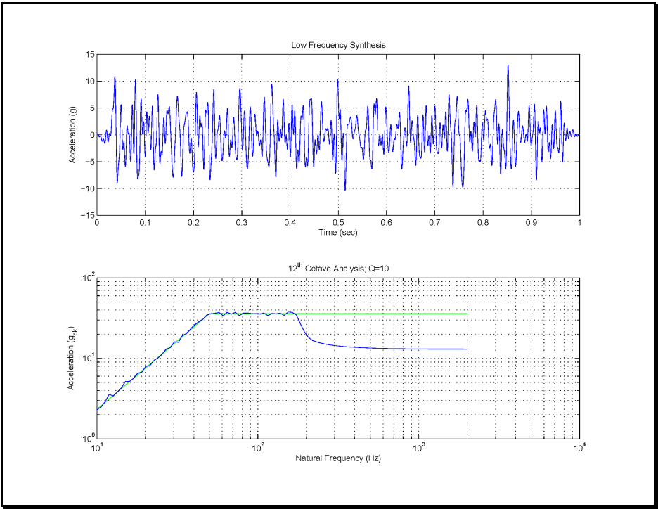
Figure description:
Acceleration Synthesis and Octave Analysis
Low Frequency Synthesis
| Time (sec) | Acceleration (g) |
|---|---|
| 0.00 | 0.0 |
| 0.02 | 1.0 |
| 0.03 | -1.5 |
| 0.04 | 11.0 |
| 0.05 | -8.5 |
| 0.08 | 10.5 |
| 0.09 | -8.0 |
| 0.12 | 7.5 |
| 0.13 | -8.5 |
| 0.16 | 7.5 |
| 0.20 | -4.5 |
| 0.21 | 8.0 |
| 0.23 | -7.0 |
| 0.25 | 8.5 |
| 0.30 | 8.5 |
| 0.33 | -7.5 |
| 0.36 | 9.5 |
| 0.45 | -6.0 |
| 0.50 | 10.5 |
| 0.52 | -10.0 |
| 0.65 | 9.0 |
| 0.67 | -6.0 |
| 0.74 | -9.5 |
| 0.81 | -7.0 |
| 0.85 | 13.0 |
| 0.91 | -8.5 |
| 1.00 | 0.0 |
12th Octave Analysis; Q=10
Legend
- Analysis (blue line — color: blue; symbol: Solid line
- Reference (green line — color: green; symbol: Solid line
| Natural Frequency (Hz) | Analysis (g_pk) | Reference (g_pk) |
|---|---|---|
| 10 | 2.5 | 2.5 |
| 15 | 5.0 | 5.0 |
| 20 | 8.0 | 8.0 |
| 30 | 15.0 | 15.0 |
| 40 | 25.0 | 25.0 |
| 50 | 35.0 | 35.0 |
| 60 | 35.0 | 35.0 |
| 70 | 37.0 | 35.0 |
| 80 | 34.0 | 35.0 |
| 90 | 36.0 | 35.0 |
| 100 | 35.0 | 35.0 |
| 120 | 34.0 | 35.0 |
| 140 | 36.0 | 35.0 |
| 160 | 34.0 | 35.0 |
| 180 | 30.0 | 35.0 |
| 200 | 21.0 | 35.0 |
| 300 | 15.5 | 35.0 |
| 400 | 14.5 | 35.0 |
| 600 | 14.0 | 35.0 |
| 1000 | 13.5 | 35.0 |
| 2000 | 13.5 | 35.0 |
Notes: The top chart displays acceleration over time, representing a low-frequency synthesis waveform. The bottom chart displays the results of a 12th-octave analysis on a log-log scale, with a target/reference curve shown in green and the actual analysis result in blue.
Figure 519.8B-4. Bandlimited random synthesis (10 Hz – 200 Hz).
Figure 519.8B-5 displays the effects of the low frequency synthesis of Figure 519.8B-4 added to the concatenated pulse in Figure 519.8B-3. The resulting time history provided in Figure 519.8B-5 is a first iteration of a possible reference to be used for the TWR testing. The lower plot in Figure 519.8B-5 displays the difference between the SRS specification and the SRS for the analytical generation to be executed under TWR as described in Method 525.2. Slight iterations on the high frequency synthesis are possible if it is determined that the original iteration is not sufficiently close to the desired reference.
Once an acceptable one second reference time history has been established, it is just a matter of programming the TWR software to repeat the one second record ten times with two seconds between each event as specified per the LCEP in the introductory paragraph of this example.
It should also be clear that the manipulation involved in this process requires that of a trained analyst. Once a reference time history has been synthesized and accepted by the appropriate test authority, the resulting time history may be used as a common reference in the event multiple laboratories are involved in conduct of a common test.
MIL-STD-810H
METHOD 519.8 ANNEX B
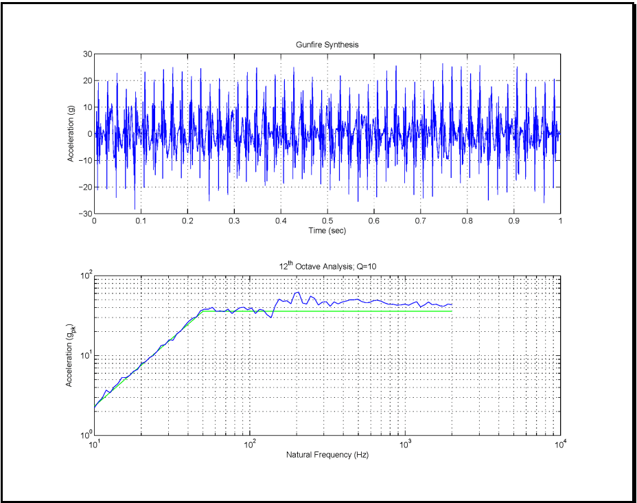
Figure description:
Gunfire Synthesis
| Time (sec) | Acceleration (g) |
|---|---|
| 0.00 | 0.0 |
| 0.02 | 19.5 |
| 0.04 | -18.2 |
| 0.06 | 16.8 |
| 0.08 | -22.5 |
| 0.10 | 21.3 |
| 0.12 | -19.8 |
| 0.15 | 23.4 |
| 0.20 | 22.1 |
| 0.25 | 20.5 |
| 0.30 | 18.2 |
| 0.35 | 22.8 |
| 0.40 | 19.4 |
| 0.45 | 24.1 |
| 0.50 | 21.6 |
| 0.55 | 17.9 |
| 0.60 | 23.5 |
| 0.65 | 25.4 |
| 0.70 | 20.8 |
| 0.75 | 26.3 |
| 0.80 | 24.2 |
| 0.85 | 25.1 |
| 0.90 | 24.8 |
| 0.95 | -26.1 |
| 1.00 | 2.5 |
12th Octave Analysis; Q=10
Legend
- Measured/Synthesized Acceleration — color: blue; symbol: Solid line
- Reference/Envelope Level — color: green; symbol: Solid line
| Natural Frequency (Hz) | Blue Line Acceleration (g_pk) | Green Line Acceleration (g_pk) |
|---|---|---|
| 10 | 2.2 | 2.2 |
| 15 | 5.5 | 4.8 |
| 20 | 8.5 | 8.0 |
| 30 | 15.2 | 16.0 |
| 40 | 26.5 | 25.0 |
| 50 | 38.0 | 35.0 |
| 60 | 41.5 | 35.0 |
| 80 | 37.0 | 35.0 |
| 100 | 42.0 | 35.0 |
| 120 | 33.0 | 35.0 |
| 150 | 53.0 | 35.0 |
| 200 | 65.0 | 35.0 |
| 300 | 48.0 | 35.0 |
| 400 | 54.0 | 35.0 |
| 500 | 52.0 | 35.0 |
| 700 | 48.0 | 35.0 |
| 1000 | 42.0 | 35.0 |
| 1500 | 46.0 | 35.0 |
| 2000 | 44.0 | 35.0 |
Notes: The first chart is a time-domain signal of synthesized gunfire. The second chart is a frequency-domain analysis (SRS or similar on log-log axes. The green line in the second chart appears to be a target envelope starting at 2.2 g at 10 Hz, increasing linearly on the log-log scale to 35 g at 50 Hz, and remaining constant thereafter up to 2000 Hz.)
Figure 519.8B-5. Synthesized one-second gunfire shock pulse train reference per additive model.
519.8 ANNEX C
519.8 ANNEX C
| 10 log10 (Tj) = 10 log10 (NF1E) + H+M+W +J+ Bj- 53 dB | |
|---|---|
| 10 log10 (Pi) = 10 log10 (T3) + Ki + 17 dB | |
| for | |
| N | Maximum number of closely spaced guns firing together. For guns that are dispersed on the host aircraft, such as in wing roots and in gun pods, separate vibration gunfire test spectra are determined for each gun location. The vibration levels, for test purposes, are selected for the gun that produces the maximum vibration levels. |
| E | Blast energy of gun (see Table 519.8C-III). |
| H | Effect of gun standoff distance, h (see Figure 519.8C-4). |
| M | Effect of gun location M = 0 unless a plane normal to the axis of the gun barrel and located at the muzzle of the gun does not intersect the aircraft structure, then M = -6 dB. |
| W | Effect of weight of the equipment to be tested (use Figure 519.8C-5). If the weight of the materiel is unknown, use W = 4.5 kilograms (10 lbs). |
| J | Effect of the materiel's location relative to air vehicle's skin (use Figures 519.8C-2 and 519.8C-6). |
| Bj | Effect of vector distance from the gun muzzle to the materiel location (see Figure 519.8C-7). |
| F1 | Gunfiring rate where F1 = fundamental frequency from Table 519.8C-II (F2 = 2F1, F3 = 3F1, F4 = 4F1) |
| Tj | Test level in g2/Hz |
| Pi | Test level for frequency Fi in g2/Hz (where i = 1 to 4) |
| Ki | Effect of vector distance on each vibration peak, Pi (see Figure 519.8C-8). |
Note: These equations are in metric units. The resultant dB values are relative to 1 g²/Hz.
MIL-STD-810H
METHOD
519.8 ANNEX C
| Aircraft/Pod | Gun (Quantity) | Location | Firing Rate | Capacity | |
|---|---|---|---|---|---|
| Rnds/Min | Rnds/Sec | ||||
| A-4 | MK12 (2) | Wing roots | 1000 | 16.6 | 100/Gun |
| A-7D | M61A1 (1) | Nose, left side | 4000 & 6000 | 66.6 & 100 | 1020 |
| A-10 | GAU-8/A (1) | Nose | 2100 & 4200 | 35 & 70 | 1175 |
| A-37 | GAU-2B/A (1) | Nose | 6000 | 100 | 1500 |
| F-4 | M61A1 (1) | Nose | 4000 & 6000 | 66.6 & 100 | 638 |
| F-5E | M39 (2) | Nose | 3000 | 50 | 300/Gun |
| F-5F | M39 (1) | Nose | 3000 | 50 | 140 |
| F-14 | M61A1 (1) | Left side of nose | 4000 & 6000 | 66.6 & 100 | 676 |
| F-15 | M61A1 (1) | Right wing root | 4000 & 6000 | 66.6 & 100 | 940 |
| F-16 | M61A1 (1) | Left wing root | 6000 | 100 | 510 |
| F-18 | M61A1 (1) | Top center of nose | 4000 & 6000 | 66.6 & 100 | 570 |
| F-111 | M61A1 (1) | Underside of fuselage | 5000 | 83.3 | 2084 |
| GEPOD 30 | GE430 (1) (GAU-8/A) | POD | 2400 | 40 | 350 |
| SUU-11/A | GAU-2B/A (1) | POD | 3000 & 6000 | 50 & 100 | 1500 |
| SUU-12/A | AN-M3 (1) | POD | 1200 | 19 | 750 |
| SUU-16/A | M61A1 (1) | POD | 6000 | 100 | 1200 |
| SUU-23/A | GAU-4/A (1) | POD | 6000 | 100 | 1200 |
| Gun | Gun Caliber, c | Blast Energy, E (J)* | |
|---|---|---|---|
| mm | in | ||
| GAU-2B/A | 7.62 | 0.30 | 6,700 |
| GAU-4/A | 20 | 0.79 | 74,600 |
| GAU-8/A | 30 | 1.18 | 307,500 |
| AN-M3 | 12.7 | 0.50 | 26,000 |
| M3 | 20 | 0.79 | 83,000 |
| M24 | 20 | 0.79 | 80,500 |
| M39 | 20 | 0.79 | 74,600 |
| M61A1 | 20 | 0.79 | 74,600 |
| MK11 | 20 | 0.79 | 86,500 |
| MK12 | 20 | 0.79 | 86,500 |
*joules (J) x 0.7376 = foot-pounds
MIL-STD-810H METHOD
519.8 ANNEX C
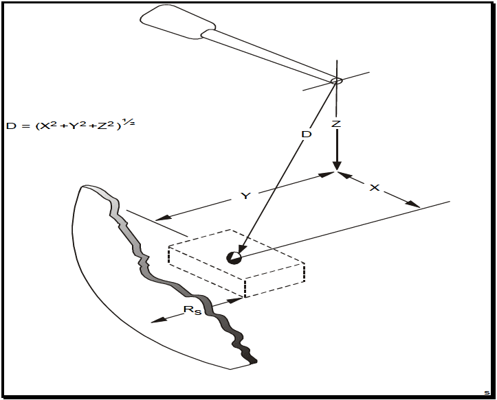
Figure description:
Figure 519.8C-2: The distance parameter (D and the depth parameter (Rs
Key Parameters and Formulas
- Distance (D: The Euclidean distance from an origin point to a target point, defined by the formula: D = (X^2 + Y^2 + Z^2^{1/2}
- Depth Parameter (: The distance between a target volume and an adjacent irregular surface.
Geometric Entities
- X, Y, Z Axes: Dimensional coordinates defining the spatial position of a target point.
- Target Volume: Represented by a dashed rectangular prism containing the target point.
- Irregular Surface: A shaded boundary located at a depth of from the target volume.
- Probe/Tool Tip: The reference point from which distance is measured.
Figure 519.8C-2. The distance parameter (D) and the depth parameter (Rs)
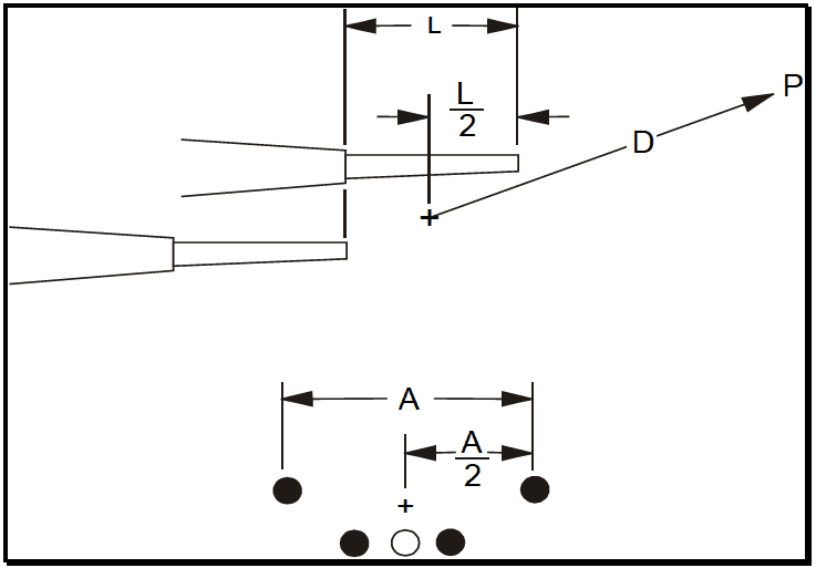
Figure description:
The image is a technical diagram illustrating the geometric parameters for a group of closely spaced guns.
Key Entities and Parameters:
- L: Length of the gun section.
- L/2: Horizontal midpoint of the gun section, indicated by a center mark (+.
- A: Total lateral width or aperture of the gun group.
- A/2: Lateral midpoint of the gun group, indicated by a center mark (+.
- D: Distance parameter measured from the central point (+ of the group to a specific point P.
- Gun Grouping: The bottom view shows a cluster of five guns (represented by circular cross-sections arranged in a specific pattern.
Figure 519.8C-3. Multiple guns, closely grouped.
MIL-STD-810H METHOD 519.8 ANNEX C
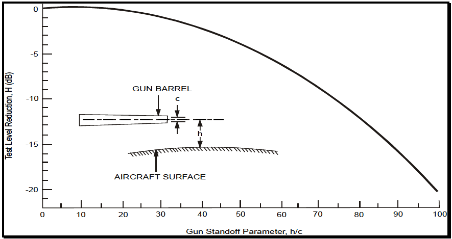
Figure description:
Gun Standoff Performance Chart
Test Level Reduction, H (dB vs. Gun Standoff Parameter, h/c
Annotations
- GUN BARREL (text_label - position: above illustration of gun barrel)
- c (text_label - position: indicates gun barrel diameter)
- h (text_label - position: indicates distance from aircraft surface to gun barrel centerline)
- AIRCRAFT SURFACE (text_label - position: below illustration of curved surface)
| Gun Standoff Parameter, h/c | Test Level Reduction, H (dB) |
|---|---|
| 0 | 0.0 |
| 10 | -0.2 |
| 20 | -0.8 |
| 30 | -1.8 |
| 40 | -3.1 |
| 50 | -5.0 |
| 60 | -7.5 |
| 70 | -10.5 |
| 80 | -14.0 |
| 90 | -17.5 |
| 100 | -20.5 |
Notes: The figure contains an illustration defining the variables: 'c' is the gun barrel diameter and 'h' is the distance between the aircraft surface and the gun barrel's longitudinal axis.
Figure 519.8C-4. Test level reduction due to gun standoff parameter.
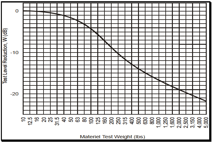
Figure description:
Test Level Reduction, W (dB as a function of Materiel Test Weight (lbs
Test Level Reduction vs. Materiel Test Weight
| Materiel Test Weight (lbs) | Test Level Reduction, W (dB) |
|---|---|
| 10 | 0.0 |
| 12.5 | -0.1 |
| 16 | -0.2 |
| 20 | -0.4 |
| 25 | -0.6 |
| 31.5 | -0.9 |
| 40 | -1.3 |
| 50 | -1.8 |
| 63 | -2.5 |
| 80 | -3.4 |
| 100 | -4.4 |
| 125 | -5.6 |
| 160 | -6.9 |
| 200 | -8.2 |
| 250 | -9.9 |
| 315 | -11.4 |
| 400 | -12.7 |
| 500 | -14.0 |
| 630 | -15.3 |
| 800 | -16.4 |
| 1,000 | -17.5 |
| 1,250 | -18.6 |
| 1,600 | -19.7 |
| 2,000 | -20.6 |
| 2,500 | -21.6 |
| 3,150 | -22.6 |
| 4,000 | -23.5 |
| 5,000 | -24.4 |
Notes: The x-axis represents 'Materiel Test Weight' in lbs on a logarithmic scale. The y-axis represents 'Test Level Reduction, W' in dB on a linear scale. Data points are estimated based on the grid provided in the chart.
Figure 519.8C-5. Test level reduction due to materiel mass loading.
MIL-STD-810H METHOD 519.8 ANNEX C
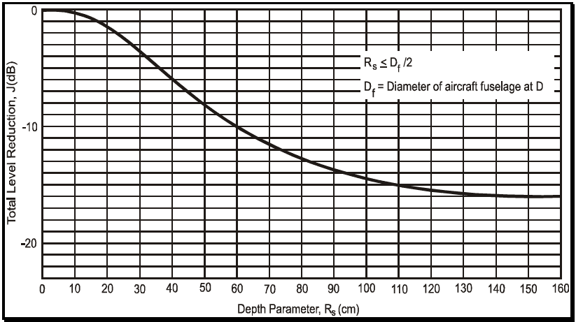
Figure description:
Total Level Reduction vs. Depth Parameter
Total Level Reduction, J(dB vs. Depth Parameter, R_s (cm
Annotations
- R_s ≤ D_f / 2 (text_label - position: x ≈ 115, y ≈ -4.2)
- D_f = Diameter of aircraft fuselage at D (text_label - position: x ≈ 115, y ≈ -6.2)
| Depth Parameter, R_s (cm) | Total Level Reduction, J(dB) |
|---|---|
| 0 | 0.0 |
| 10 | -0.4 |
| 20 | -1.6 |
| 30 | -3.8 |
| 40 | -6.4 |
| 50 | -8.8 |
| 60 | -10.8 |
| 70 | -12.4 |
| 80 | -13.7 |
| 90 | -14.7 |
| 100 | -15.4 |
| 110 | -15.9 |
| 120 | -16.2 |
| 130 | -16.4 |
| 140 | -16.5 |
| 150 | -16.5 |
| 160 | -16.5 |
Notes: The graph illustrates a non-linear relationship where the Total Level Reduction (J decreases (becomes more negative as the Depth Parameter (R_s increases. The reduction starts at 0 dB for R_s = 0 and plateaus at approximately -16.5 dB for R_s values of 140 cm and beyond. The chart includes conditions for the depth parameter relative to the aircraft fuselage diameter.)))
Figure 519.8C-6. Test level reduction due to depth parameter.
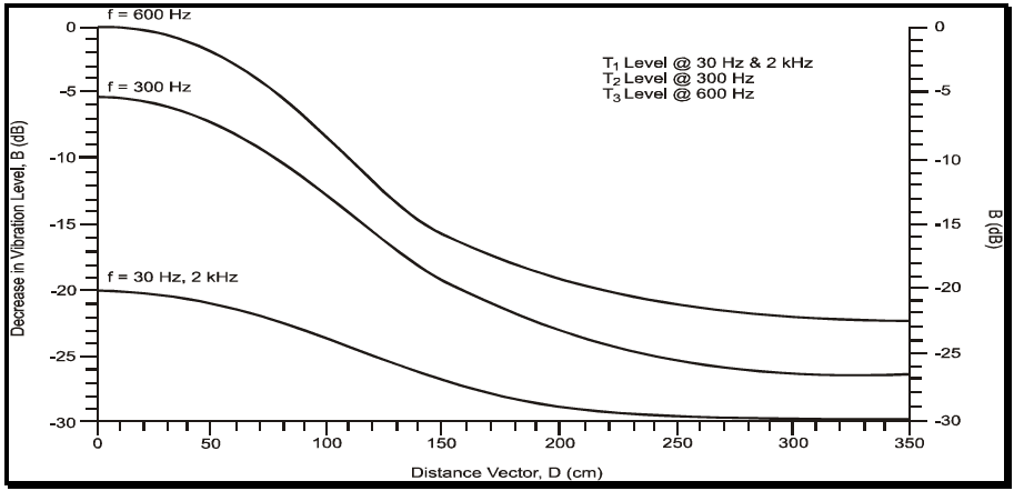
Figure description:
Decrease in Vibration Level vs. Distance
Decrease in Vibration Level, B (dB vs. Distance Vector, D (cm
Legend
- T1 Level @ 30 Hz & 2 kHz — color: black; symbol: Solid line
- T2 Level @ 300 Hz — color: black; symbol: Solid line
- T3 Level @ 600 Hz — color: black; symbol: Solid line
| Distance Vector, D (cm) | f = 600 Hz (dB) | f = 300 Hz (dB) | f = 30 Hz, 2 kHz (dB) |
|---|---|---|---|
| 0 | 0.0 | -5.5 | -20.0 |
| 25 | -0.5 | -6.0 | -20.2 |
| 50 | -2.0 | -7.5 | -21.0 |
| 75 | -5.0 | -10.0 | -22.5 |
| 100 | -9.0 | -14.0 | -25.0 |
| 125 | -13.0 | -17.5 | -27.0 |
| 150 | -16.0 | -20.5 | -28.5 |
| 175 | -18.5 | -22.5 | -29.5 |
| 200 | -20.0 | -24.0 | -29.8 |
| 225 | -21.0 | -25.0 | -30.0 |
| 250 | -21.5 | -25.5 | -30.0 |
| 275 | -22.0 | -26.0 | -30.0 |
| 300 | -22.2 | -26.3 | -30.0 |
| 325 | -22.4 | -26.4 | -30.0 |
| 350 | -22.5 | -26.5 | -30.0 |
Notes: The chart shows three curves representing decrease in vibration level (B in dB relative to distance (D in cm for different frequencies. The curves are also labeled as T1, T2, and T3 levels in the top right text block.))
Figure 519.8C-7. Decrease in vibration level with vector distance from gun muzzle.
MIL-STD-810H METHOD
519.8 ANNEX C
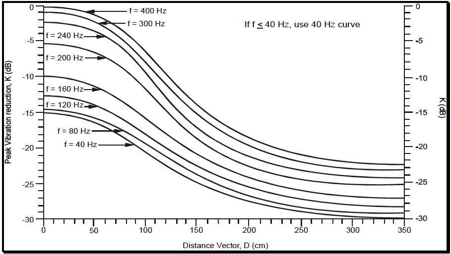
Figure description:
Vibration Reduction Curves for Different Frequencies
Peak Vibration reduction, K (dB vs Distance Vector, D (cm
Legend
- f = 400 Hz — color: black; symbol: solid line
- f = 300 Hz — color: black; symbol: solid line
- f = 240 Hz — color: black; symbol: solid line
- f = 200 Hz — color: black; symbol: solid line
- f = 160 Hz — color: black; symbol: solid line
- f = 120 Hz — color: black; symbol: solid line
- f = 80 Hz — color: black; symbol: solid line
- f = 40 Hz — color: black; symbol: solid line
Annotations
- If f ≤ 40 Hz, use 40 Hz curve (text_label - position: top right quadrant)
| Distance Vector, D (cm) | f = 400 Hz (dB) | f = 300 Hz (dB) | f = 240 Hz (dB) | f = 200 Hz (dB) | f = 160 Hz (dB) | f = 120 Hz (dB) | f = 80 Hz (dB) | f = 40 Hz (dB) |
|---|---|---|---|---|---|---|---|---|
| 0 | 0.0 | -1.0 | -2.2 | -5.5 | -10.0 | -12.8 | -14.5 | -15.2 |
| 25 | -0.1 | -1.1 | -2.4 | -5.7 | -10.2 | -13.0 | -14.7 | -15.5 |
| 50 | -0.5 | -1.5 | -3.2 | -6.5 | -11.0 | -13.8 | -15.5 | -16.2 |
| 75 | -2.5 | -3.8 | -5.8 | -9.0 | -13.0 | -15.5 | -17.0 | -17.8 |
| 100 | -6.0 | -7.5 | -9.5 | -12.5 | -15.5 | -17.5 | -19.0 | -20.0 |
| 125 | -10.2 | -11.5 | -13.5 | -16.0 | -18.8 | -20.5 | -22.0 | -23.0 |
| 150 | -14.0 | -15.0 | -16.5 | -19.0 | -21.5 | -22.8 | -24.5 | -25.5 |
| 175 | -16.5 | -17.8 | -18.8 | -21.0 | -23.2 | -24.5 | -26.2 | -27.2 |
| 200 | -18.5 | -19.5 | -20.5 | -22.5 | -24.5 | -25.5 | -27.5 | -28.5 |
| 225 | -20.2 | -21.2 | -22.2 | -24.0 | -25.8 | -26.8 | -28.2 | -29.0 |
| 250 | -21.5 | -22.5 | -23.5 | -25.0 | -26.5 | -27.5 | -28.5 | -29.2 |
| 275 | -21.8 | -22.8 | -24.0 | -25.5 | -26.8 | -27.8 | -28.8 | -29.5 |
| 300 | -22.0 | -23.0 | -24.2 | -25.8 | -27.0 | -28.0 | -29.0 | -29.8 |
| 325 | -22.1 | -23.1 | -24.3 | -25.9 | -27.1 | -28.1 | -29.1 | -29.9 |
| 350 | -22.2 | -23.2 | -24.4 | -26.0 | -27.2 | -28.2 | -29.2 | -30.0 |
Notes: The graph shows vibration reduction (K as a function of distance (D for various frequencies (f. All curves follow a similar sigmoidal shape, with reduction increasing (more negative K as distance increases and frequency decreases. The Y-axis represents Peak Vibration reduction K in dB, and the X-axis represents Distance Vector D in cm.))))
Figure 519.8C-8. Gunfire peak vibration reduction with distance.
The key geometrical relations used to determine the predicted vibration spectra are the following four geometrical factors:
- a. Vector distance (D). The vector distance from the muzzle of the gun to the mean distance between materiel support points as shown on Figure 519.8C-2. For configurations involving multiple guns, the origin of vector D is determined from the centroidal point of the gun muzzle, as shown on Figure 519.8C- 3. Figure 519.8C-7 and Figure 519.8C-8 provide for spectra reduction factors related to D for the random spectra and the discrete frequency spectra, respectively.
- b. Gun standoff distance (h). The distance normal to the aircraft's surface as shown on Figure 519.8C-4.
- c. Depth parameter (Rs). The distance normal to the aircraft's skin to the materiel location inside the aircraft. If Rs is unknown, use Rs = 7.6 cm (3 in.) (see Figure 519.8C-2). Figure 519.8C-6 provides spectra reduction factors related to Rs.
- d. Gun caliber. Table 519.8C-III defines the gun caliber parameter, c, in millimeters and inches. For this procedure, base the vibration peak bandwidths consistent with windowed Fourier processing on in-service measured materiel response data if available. When such in-service data are not available, the vibration peak bandwidths can be calculated as:
For cases where the gun firing rate changes during a development program or the gun may be fired at a sweep rate, it is desirable to either (1) perform sinusoidal sweeps within the proposed bandwidth for the fundamental and each harmonic, or (2) apply narrowband random vibration levels provided the sweep frequency bandwidth is not too large. This technique may over-predict those frequencies where the attachment structure or materiel responses become significantly nonlinear. Likewise, for those cases in which the attachment structure or materiel resonances coincide with the frequencies in the gunfire environment, the materiel vibration response could be under-predicted. The practitioner should clearly understand the options available and inherent limitations in the vibration control system software.