516.8-4 SHOCK IDENTIFICATION AND ANOMALOUS MEASUREMENT BEHAVIOR
In the course of examination of some 216 mechanical shocks from a single test series (reference paragraph 6.1.c) the variation in time history form is substantial, and requires the judgment of an analyst for development of a specification for which shock synthesis for an electrodynamic exciter might be appropriate. Figures 516.8B-7 through 9 display typical anomalous time histories related to signal conditioning or transducer problems. The identification of the problem is assumed, and generally based upon a visual examination of the time history.
MIL-STD-810H METHOD 516.8 ANNEX B
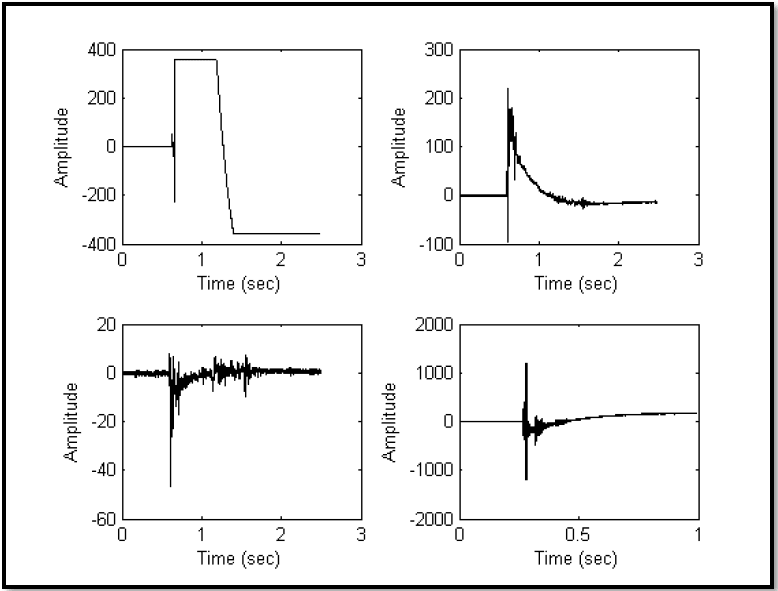
Figure description:
Waveform Amplitude over Time
Top-left Plot
| Time (sec) | Amplitude |
|---|---|
| 0.0 | 0.0 |
| 0.65 | 0.0 |
| 0.66 | -230.0 |
| 0.67 | 360.0 |
| 1.15 | 360.0 |
| 1.4 | -360.0 |
| 2.5 | -360.0 |
Top-right Plot
| Time (sec) | Amplitude |
|---|---|
| 0.0 | 0.0 |
| 0.6 | 0.0 |
| 0.61 | -100.0 |
| 0.62 | 220.0 |
| 0.7 | 80.0 |
| 1.0 | 25.0 |
| 1.5 | -20.0 |
| 2.0 | -20.0 |
| 2.5 | -15.0 |
Bottom-left Plot
| Time (sec) | Amplitude |
|---|---|
| 0.0 | 0.0 |
| 0.58 | 0.0 |
| 0.6 | -47.0 |
| 0.62 | 8.0 |
| 0.7 | -5.0 |
| 1.0 | -1.0 |
| 1.2 | 6.0 |
| 1.5 | 8.0 |
| 1.7 | -3.0 |
| 2.5 | 2.0 |
Bottom-right Plot
| Time (sec) | Amplitude |
|---|---|
| 0.0 | 0.0 |
| 0.28 | 0.0 |
| 0.29 | -1200.0 |
| 0.3 | 1200.0 |
| 0.35 | -300.0 |
| 0.4 | -50.0 |
| 0.6 | 100.0 |
| 0.8 | 160.0 |
| 1.0 | 180.0 |
Notes: The figure contains four separate plots showing Amplitude vs Time (sec for different signals. Each plot captures a pulse or spike event occurring at a specific time followed by a decay or steady-state behavior.)
Figure 516.8B-7. Measurement input overdriving the signal conditioning with clipping.
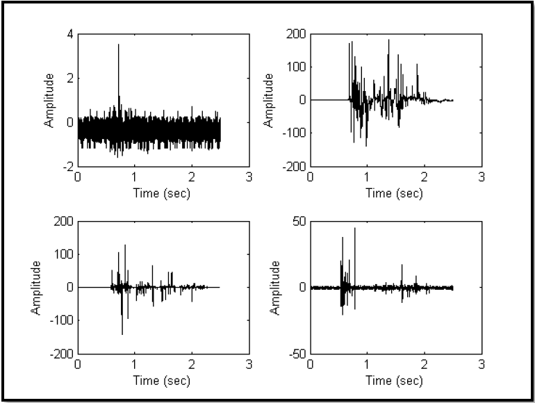
Figure description:
Top-Left Chart
| Time (sec) | Amplitude |
|---|---|
| 0.0 | -0.1 |
| 0.2 | 0.2 |
| 0.4 | -0.3 |
| 0.6 | 0.1 |
| 0.73 | 3.5 |
| 0.8 | -0.4 |
| 1.0 | 0.2 |
| 1.5 | -0.1 |
| 2.0 | 0.3 |
| 2.5 | 0.0 |
Top-Right Chart
| Time (sec) | Amplitude |
|---|---|
| 0.0 | 0 |
| 0.6 | 0 |
| 0.7 | 175 |
| 0.8 | -120 |
| 0.9 | 180 |
| 1.0 | 50 |
| 1.4 | 180 |
| 1.6 | 120 |
| 1.9 | 110 |
| 2.2 | 10 |
| 2.5 | 0 |
Bottom-Left Chart
| Time (sec) | Amplitude |
|---|---|
| 0.0 | 0 |
| 0.6 | 0 |
| 0.7 | 110 |
| 0.8 | -140 |
| 0.9 | 130 |
| 1.3 | 70 |
| 1.6 | 50 |
| 2.1 | 20 |
| 2.5 | 0 |
Bottom-Right Chart
| Time (sec) | Amplitude |
|---|---|
| 0.0 | 1 |
| 0.5 | -2 |
| 0.6 | 40 |
| 0.7 | -30 |
| 0.8 | 45 |
| 1.6 | 18 |
| 1.9 | 10 |
| 2.5 | 1 |
Notes: The figure consists of four subplots displaying time-series waveforms. Each chart has Time (sec on the x-axis ranging from 0 to 3, and Amplitude on the y-axis with varying scales.)
Figure 516.8B-8. Noisy or missing measurement signals.
MIL-STD-810H METHOD 516.8 ANNEX B
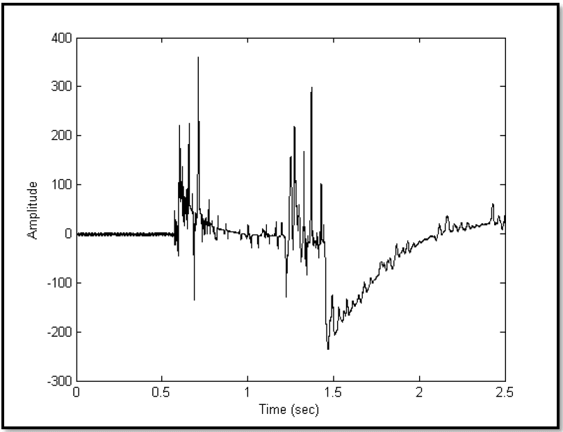
Figure description:
| Time (sec) | Amplitude |
|---|---|
| 0.00 | 0 |
| 0.10 | 0 |
| 0.20 | 0 |
| 0.30 | 0 |
| 0.40 | 0 |
| 0.50 | 0 |
| 0.55 | 0 |
| 0.58 | 50 |
| 0.60 | 220 |
| 0.61 | -40 |
| 0.63 | 100 |
| 0.65 | 180 |
| 0.67 | 230 |
| 0.69 | -135 |
| 0.72 | 360 |
| 0.75 | 40 |
| 0.80 | 30 |
| 0.85 | 50 |
| 0.90 | 10 |
| 1.00 | 5 |
| 1.10 | -5 |
| 1.20 | -80 |
| 1.25 | 155 |
| 1.28 | 215 |
| 1.30 | -20 |
| 1.33 | 165 |
| 1.35 | -80 |
| 1.38 | 295 |
| 1.40 | -20 |
| 1.43 | 100 |
| 1.46 | -235 |
| 1.50 | -160 |
| 1.60 | -170 |
| 1.70 | -120 |
| 1.80 | -100 |
| 1.90 | -60 |
| 2.00 | -40 |
| 2.10 | -10 |
| 2.15 | 35 |
| 2.20 | 10 |
| 2.30 | 15 |
| 2.40 | 25 |
| 2.45 | 60 |
| 2.50 | 20 |
Notes: The data extracted represents key peaks and shifts in a noisy signal shown over time. The amplitude is measured in arbitrary units on the y-axis, and time is measured in seconds on the x-axis.
Figure 516.8B-9. Combination amplifier overdriving and noise.
Based on similar displays, all of these time histories must be rejected and the source of the problem identified before continuing to make measurements. Figure 516.8B-8 illustrates noise in the system that could be from a loose connector or even a missing sensor. Once again, measurement time histories of this form need to be rejected. Measurement time histories with a few clearly identified noise “spikes” may often be “corrected” by a trained analyst and used.
Finally, Figure 516.8B-9 illustrates a combination of amplifier over driving and noise corruption. Once again, this measurement must be rejected.
Downloaded from https://www.everyspec.com
MIL-STD-810H
METHOD 516.8 ANNEX B
(This page is intentionally blank.)
MIL-STD-810H
METHOD 516.8 ANNEX C METHOD 516.8, ANNEX C STATISTICAL AND PROBABILISTIC CONSIDERATIONS FOR DEVELOPING LIMITS ON PREDICTED AND PROCESSED DATA ESTIMATES
516.8-4 RECOMMENDED PROCEDURES
4.1 Test Facility
Use a shock-producing apparatus capable of meeting the test conditions as determined according to the appropriate paragraphs of this Method. The shock apparatus may be of the free fall, resilient rebound, non-resilient rebound, hydraulic, compressed gas, electrodynamic exciter, servo-hydraulic exciter, or other capable configuration. Careful attention needs to be paid to the time, amplitude, and frequency ranges over which the apparatus is capable of
MIL-STD-810H
METHOD 516.8
delivering a shock input. For example, electrodynamic exciters can suitably reproduce synthesized shock records from 5 Hz to 2000 Hz or above; however, a servo-hydraulic exciter may have only a DC to 500 Hz controllable frequency range. Procedures II and III require test apparatus capable of producing relatively large displacement. Procedure VII is a special test setup in that large containers impact a rigid barrier. Procedure VIII for catapult launch is best satisfied by application of two shock pulses with an intervening “transient vibration” for which TWR Method 525.2 may be appropriate. Generally, shock on either electrodynamic or servo-hydraulic exciters will be controlled using classical shock, SRS shock, or time waveform replication control software.
516.8-4.1 Recommended Statistical Procedures for Upper Limit Estimates
Paragraph 6.1, reference b, provides a detailed discussion of the advantages and disadvantages of estimate upper limits. The guidelines in this reference are recommended. In all cases, plot the data carefully with a clear indication of the method of establishing the upper limit and the assumptions behind the method used.
- a. When N is sufficiently large, i.e., N > 7, establish the upper limit by using the expression for the DFL for a selected β > 0.90 such that γ > 0.50.
- b. When N is not sufficiently large to meet the criterion in (a), establish the upper limit by using the expression for the NTL. Select β and γ ≥ 0.50. Variation in β will determine the degree of conservativeness of the upper limit.
- c. For N > 10 and a confidence coefficient of 0.50, the upper limit established on the basis of ETL is acceptable and may be substituted for the upper limit established by DFL or NTL. It is important when using ETL to examine and confirm the homogeneity of the estimates over the frequency bands.
4.2 Controls
516.8-4.2 Uncertainty Factors
Uncertainty factors may be added to the resulting upper limits if confidence in the data is low or the data set is small. Factors on the order of 3 dB to 6 dB may be added. Paragraph 6.1, reference b recommends a 5.8 dB uncertainty factor (based on “flight-to-flight” uncertainties of 3 dB, and “point-to-point” uncertainties of 5 dB) be used with captive carry flight measured data to determine a maximum expected environment using a normal tolerance limit. It is important that all uncertainties be clearly defined, and that uncertainties are not superimposed upon estimates that already account for uncertainty.
MIL-STD-810H METHOD
4.2.1 Calibration
The shock apparatus will be user-calibrated for conformance with the specified test requirement from the selected procedure where the response measurements will be made with traceable laboratory calibrated measurement devices. Conformance to test specifications may require use of a “calibration load” in the test setup. If the calibration load is required, it will generally be a mass/stiffness simulant of the test item. “Mass/stiffness simulants” imply that the modal dynamic characteristics of the test item are replicated to the extent possible in the simulant - particularly those modal dynamic characteristics that may interact with the modal dynamic configuration of the fixturing and/or the test device. For calibration, produce two consecutive input applications to a calibration load that satisfy the test conditions outlined in Procedures I, II, III, V, or VIII. After processing the measured response data from the calibration load, and verifying that it is in conformance with the test specification tolerances, remove the calibration load and perform the shock test on the test item. Use of calibration loads for setup to guard against excessive over test or unproductive under test is highly recommended in all cases.
4.2.2 Tolerances
For test validation, use the tolerances specified under each individual procedure, along with the guidelines provided below. In cases in which such tolerances cannot be met, establish achievable tolerances that are agreed to by the cognizant engineering authority and the customer prior to initiation of test. In cases, in which tolerances are established independently of the guidance provided below, establish these tolerances within the limitations of the specified measurement calibration, instrumentation, signal conditioning, and data analysis procedures.
4.2.2.1 Classical Pulses and Complex Transient Pulses-Time Domain
For the classical pulses in this Method, tolerance limits on the time domain representation of the pulses are as specified in Figures 516.8-3 through 516.8-5. If a classical shock pulse is defined in lieu of more complex measured time history data it must be demonstrated that SRS estimates of the classical shock pulse are within the tolerances established for the SRS estimates of the measured time history data. For complex transient pulses specified in the time domain, it is assumed that testing will be performed under TWR (Method 525.2), and that the tolerance guidance related to that Method will be used.
4.2.2.2 Complex Transient Pulses-SRS
For a complex transient pulse specified by way of the maximax SRS, e.g., Figure 516.8-2, the frequency domain and time domain tolerances are specified in terms of a tolerance on the SRS amplitude values over a specified frequency bandwidth and a tolerance on the effective pulse duration. If a series of shocks are performed, all acceleration maximax SRS shall be computed at the center frequency of one-twelfth octave bands with a default damping quality factor Q of 10 (5 percent critical damping factor). Tolerances on the individual points (values associated with each one-twelfth octave center frequency) are to be within -1.5 dB and +3 dB over a minimum of 90 percent of the overall values in the frequency bandwidth from 10 Hz to 2000 Hz. For the remaining part of the frequency band, all SRS values are to be within -3 dB and +6 dB (this places a comparatively narrow tolerance on the major frequency band of interest, but allows a wider tolerance on 10 percent of this frequency band and a wider tolerance on the SRS above 2 KHz). Note that if an SRS is within tolerance for both SRS-minimum and SRS-maximums, the pulse is considered symmetric. While the reference criteria is often limited in bandwidth as a result of excitation equipment limitations, the analyst may require response data to be viewed through the bandwidth at which the SRS amplitude flattens. The duration of the complex transient is defined by and as discussed in Annex A paragraph 1.3 and shall have a tolerance of . In addition, the following guidance is provided for use of (1) the pseudo-velocity response spectra, and (2) multiple measurements to specify a shock environment.
- a. All tolerances are specified on the maximax acceleration SRS. Any tolerances specified on the pseudo-velocity response spectra must be derived from the tolerances on the maximax acceleration SRS. (For three-coordinate paper, the pseudo-velocity tolerance can be determined by placing tolerance bands along the SRS acceleration axis, and then extracting the tolerance values along the ordinate for the pseudo-velocity SRS tolerance.) Note that SRS estimates scale directly in amplitude, i.e., multiplication of the time history by a factor is translated directly into multiplication of the SRS estimate by the same factor.
- b. The test tolerances are stated in terms of a single measurement tolerance, i.e., each individual laboratory test must fit within the tolerance bands to provide a satisfactory test. For an array of measurements defined in terms of a "zone" (paragraph 6.1, reference b), amplitude tolerance may be specified in terms of an average of the measurements within a "zone". However, this is, in effect, a relaxation of the single measurement tolerance in that individual measurements may be substantially out of tolerance while the average is within tolerance. In general, when specifying test tolerances based on averaging for more than two measurements within a zone, the tolerance band should not exceed the 95/50 one-sided normal tolerance upper limit computed for the logarithmically transformed SRS estimates, nor be less than the mean minus 1.5 dB. Any use of "zone" tolerances and averaging must have support documentation prepared by a trained analyst. The tolerance on the duration of the test pulse when more than one measurement is present, may be specified either as a percentage of the harmonic mean of the pulses (the nth root of the product of the n durations as defined by T E j for j = 1,2,..., i.e., n T E = n ∏ j=1 n ET ), or on some statistical based measure taking account of
the variance of the effective durations. For example, a 95/50 two-sided normal tolerance limit will provide the upper and lower limits of duration for which it is expected that 95 percent of future measurements will fall with 50 percent confidence coefficient. 10 percent of the difference in these limits might be a reasonable duration tolerance. For further possible ways of statistically defining specification of duration tolerance see Annex C).
- c. If the test item has no significant low frequency modal response, it is permissible to allow the low frequency portion of the SRS to fall out of tolerance in order to satisfy the high frequency portion of the SRS, provided the high frequency portion begins at least one octave below the first natural mode frequency, 1f , of the mounted test item. Recall that f min was defined to be one octave below 1f . The reference pulse synthesis should be conducted such that as much of the spectrum below f min remains in tolerance as possible without exceeding the specified duration T . E
- d. If the test item has significant low frequency modal response, it is permissible to allow the duration of the complex transient pulse to fall outside of the range (provided in Table 516.8-III), in order to satisfy the low frequency portion of the SRS. The effective duration contained in Table 516.8-III may be increased by as much as in addition to , (e.g., ), in order to have the low frequency portion of the SRS within tolerance. If the duration of the complex transient pulse must exceed in order to have the low frequency portion of the SRS within tolerance, use a new shock procedure.
4.3 Test Interruption
Test interruptions can result from two or more situations, one being from malfunction of the shock apparatus or associated laboratory test support equipment. The second type of test interruption results from malfunction of the test item itself during operational checks.
4.3.1 Interruption Due To Laboratory Equipment Malfunction
- a. General. See Part One, paragraph 5.11 of this Standard.
- b. Specific to this Method. Interruption of a shock test sequence is unlikely to generate any adverse effects. Normally, continue the test from the point of interruption.
4.3.2 Interruption Due To Test Item Operation Failure
Failure of the test item(s) to function as required during operational checks presents a situation with several possible options.
MIL-STD-810H
METHOD 516.8
- a. The preferable option is to replace the test item with a “new” one and restart from Step 1.
- b. A second option is to repair the failed or non-functioning component or assembly of the test item with one that functions as intended, and restart the entire test from Step 1.
NOTE: When evaluating failure interruptions, consider prior testing on the same test item, and consequences of such.
4.4 Instrumentation
In general, acceleration will be the quantity measured to meet a specification, with care taken to ensure acceleration measurements can be made that provide meaningful data. Always give special consideration to the measurement instrument amplitude and frequency range specifications in order to satisfy the calibration, measurement and analysis requirements. With regard to measurement technology, accelerometers, strain gages and laser Doppler vibrometers are commonly used devices for measurement. In processing shock data, it is important to be able to detect anomalies. For example, it is well documented that accelerometers may offset or zero-shift during mechanical shock, pyroshock, and ballistic shock (paragraph 6.1, references m, n, and s). Additional discussion on this topic is found in the pyro shock and ballistic shock methods. A part of this detection is the integration of the acceleration amplitude time history to determine if it has the characteristics of a physically realizable velocity trace. For mechanical shock various accelerometers are readily available which may or may not contain mechanical isolation. Transducer performance continues to improve with time, however, inventories across all laboratories may not be of the latest generation, and thereby making detailed calibrations critical in understanding individual transducer performance.
- a. Accelerometers. Ensure the following:
- (1) Amplitude Linearity: It is desired to have amplitude linearity within 10 percent over the entire operating range of the device. Since accelerometers (mechanically isolated or not) may show zero-shift (paragraph 6.1, reference o), there is risk in not characterizing these devices over their entire amplitude range. To address these possible zero-shifts, high pass filtering (or other data correction technique) may be required. Such additional post-test correction techniques increases the risk of distorting the measured shock environment. Consider the following in transducer selection:
(a) It is recognized that accelerometers may have both non-linear amplification and non-linear frequency content below 10,000 Hz (paragraph 6.1, reference o). In order to understand the non-linear amplification and frequency characteristics, it is recommended that shock linearity evaluations be conducted at intervals of 20 to 30 percent of the rated amplitude range (inclusive of the maximum rated range) of the accelerometer to identify the actual amplitude and frequency linearity characteristics and useable amplitude and frequency range. If a shock based calibration technique is employed, the shock pulse duration for the evaluation is calculated as:
Where TD is the duration (baseline) of the acceleration pulse and fmax is the maximum specified frequency range for the accelerometer. For mechanical shock, the default value for fmax is 10,000 Hz.
(b) For cases in which response below 2 Hz is desired, a piezoresistive accelerometer measurement is required.
- (2) Frequency Response: A flat response within ± 5 percent across the frequency range of interest is required. Since it is generally not practical or cost effective to conduct a series of varying pulse width shock tests to characterize frequency response, a vibration calibration is typically employed. For the case of a high range accelerometer with low output, there may be SNR issues associated with a low level vibration calibration. In such cases a degree of engineering judgment will be required in the
evaluation of frequency response with a revised requirement for flat frequency response to be within ± 1 dB across the frequency range of interest.
- (3) Accelerometer Sensitivity: The sensitivity of a shock accelerometer is expected to have some variance over its large amplitude dynamic range.
(a) If the sensitivity is based upon the low amplitude vibration calibration, it is critical that the linearity characteristics of the shock based “Amplitude Linearity” be understood such that an amplitude measurement uncertainty is clearly defined.
(b) Ideally, vibration calibration and shock amplitude linearity results should agree within 10 percent over the amplitude range of interest for a given test.
- (4) Transverse sensitivity should be less than or equal to 7 percent.
- (5) The measurement device and its mounting will be compatible with the requirements and guidelines provided in paragraph 6.1, reference a.
- (6) Piezoelectric or piezoresistive accelerometers may be used for mechanical shock in scenarios in which levels are known to be within the established (verified through calibration) operating range of the transducer, thereby avoiding non-linear amplification and frequency content.
b. Other Measurement Devices
- (1) Any other measurement devices used to collect data must be demonstrated to be consistent with the requirements of the test, in particular, the calibration and tolerance information provided in paragraph 4.2.
- (2) Signal Conditioning. Use only signal conditioning that is compatible with the instrumentation requirements of the test, and is compatible with the requirements and guidelines provided in paragraph 6.1, reference a. In particular, filtering of the analog voltage signals will be consistent with the time history response requirements (in general, demonstrable linearity within ± 5° of phase throughout the desired frequency domain of response), and the filtering will be so configured that anomalous acceleration data caused by clipping will not be misinterpreted as response data. In particular, use extreme care in filtering the acceleration signals at the amplifier output. Never filter the signal into the amplifier for fear of filtering erroneous measurement data, and the inability to detect the erroneous measurement data. The signal from the signal conditioning must be anti-alias filtered before digitizing as defined in Annex A paragraph 1.1.
4.5 Data Analysis
- a. In subsequent processing of the data, use any additional digital filtering that is compatible with the anti-alias analog filtering. In particular, additional digital filtering must maintain phase linearity for processing of shock time histories. Re-sampling for SRS computational error control is permitted using standard re-sampling algorithms.
- b. Analysis procedures will be in accordance with those requirements and guidelines provided in paragraph 6.1, reference a. In particular, validate the shock acceleration amplitude time histories according to the procedures in paragraph 6.1, reference a. Use integration of time histories to detect any anomalies in the measurement system, e.g., cable breakage, amplifier slew rate exceedance, data clipped, unexplained accelerometer offset, etc., before processing the response time histories. If anomalies are detected, discard the invalid measured response time history. For unique and highly valued measured data, a highly trained analyst may be consulted concerning the removal of certain anomalies but, generally, this will leave information that is biased by the technique for removal of the anomaly.
MIL-STD-810H
METHOD 516.8
4.6 Test Execution
4.6.1 Preparation for Test
Test preparation details will be procedure specific as discussed in the previous paragraphs. Ensure that all test specific equipment such as fixturing, environmental conditioning equipment, instrumentation and acquisition equipment has been properly calibrated, validated and documented.
4.6.1.1 Preliminary Guidelines
Prior to initiating any testing, review the pretest information in the test plan to determine test details (e.g., procedure, calibration load, test item configuration, measurement configuration, shock level, shock duration, climatic conditions, and number of shocks to be applied, as well as the information in paragraph 3.1 above). Note all details of the test validation procedures.
4.6.1.2 Pretest Checkout
After calibration of the excitation input device and prior to conducting the test, perform a pretest checkout of the test item at standard ambient conditions (Part One, paragraph 5.1.a) to provide baseline data. Conduct the checkout as follows:
Step 1 Conduct a complete visual examination of the test item with special attention to stress areas or areas identified as being particularly susceptible to damage and document the results.
Step 2 Where applicable, install the test item in its test fixture.
Step 3 Conduct a test item operational check in accordance with the approved test plan, and document the results for compliance with Part One, paragraph 5.15.
Step 4 If the test item operates satisfactorily, proceed to the first test. If not, resolve the problem and restart at Step 1.
4.6.1.3 Procedures' Overview
Paragraphs 4.6.2 through 4.6.9 provide the basis for collecting the necessary information concerning the system under shock. For failure analysis purposes, in addition to the guidance provided in Part One, paragraph 5.14, each procedure contains information to assist in the evaluation of the test results. Analyze any failure of a test item to meet the requirements of the system specifications, and consider related information such as follows in paragraphs 4.6.2 through 4.6.9. It is critical that any deviations to the test or test tolerances must be approved by the appropriate test authority and must be clearly documented in the test plan and final report.
4.6.2 Functional Shock (Procedure I)
The intent of this test is to disclose materiel malfunction that may result from shocks experienced by materiel during use in the field. Even though materiel may have successfully withstood even more severe shocks during shipping or transit shock tests, there are differences in support and attachment methods, and in functional checking requirements that make this test necessary. Tailoring of the test is required when data are available, can be measured, or can be estimated from related data using accepted dynamic scaling techniques (for scaling guidance see Method 525.2). When measured field data are not available for tailoring, use the information in Figure 516.8-2 and the accompanying Table 516.8-III to define the shock test system input SRS or Tables 516.8-IV-VI for classical pulse definitions. In the calibration procedure, the calibration load will be subject to a properly compensated complex waveform in accordance with the SRS described above for electrodynamic or servo-hydraulic shock testing. In general, tests using classical pulses, e.g., terminal peak sawtooth, etc., are unacceptable unless it can be demonstrated during tailoring that the field shock environment time trace approximates such a form. If all other testing resources have been exhausted, it will be permissible to use the information on Table 516.8-IV-VI for employing a classical pulse. However, such testing must be performed in both a positive and negative direction to assure meeting the spectrum requirements on Figure 516.8- 2 in both the positive and negative direction.
| Reference Peak Value and Pulse Duration | ||||||
|---|---|---|---|---|---|---|
| Test | Am (G-Pk) & TD (ms) | |||||
| Flight Vehicle Materiel¹ | Weapon Launch¹,² Captive Carry | Ground Materiel¹,³ | ||||
| Procedure I - Functional | 20 G | 11 ms | 30 G | 11 ms | 40 G | 11 ms |
Note 1. For material that is shock mounted or weighing more than 136 kg (300 lbs), an 11 ms half-sine pulse of such amplitude that yields an equivalent velocity to the default terminal peak sawtooth may be employed. Equivalent Velocity Relationship:
Note 2. Launch Shock is a special case of Functional Shock (see paragraph 6.1k)
Note 3. For materiel mounted only in trucks and semi-trailers, use a 20G peak value.
A special category of functional shock has been established for Navy high speed craft (HSC). Tables 516.8-V and 516.8-VI document two functional standardized laboratory shock test requirements to mitigate the risk of equipment malfunction or failure of hard mounted electrical and electronics equipment in HSC due to wave impacts (reference paragraph 6.1, reference p). These test requirements are applicable for equipment with internal vibration mounts, but not applicable for equipment on shock mounts (paragraph 6.1, reference q) or for shock isolated seats (paragraph 6.1, reference r).
Two types of half-sine shock tests are required to minimize the risk of equipment malfunction or failure in HSC. The first test, (HSC-I), is to be repeated three times in each direction of the three mutually orthogonal axes. The second test, (HSC-II), employs a lower severity shock pulse which is to be repeated 800 times in each direction per axis with the nominal spacing between pulses set at 1-second intervals (in the event the previous transient has not completely decayed within the nominal 1-second, contact the proper test authority for further guidance).
HSC equipment orientation during testing should represent realistic conditions in which the equipment may experience wave impact shock. Dominant wave impact shock loads occur only in craft axes +Z (vertical up), -X (aft), and +/- Y (port/starboard). Equipment that can be installed in any orientation should be tested in positive and negative test orientations for all three equipment axes. The +X and -Z craft orientations should be omitted during Procedure I testing for equipment installed only in a vertical up orientation.
| Test² | Half-Sine Pulse | |
|---|---|---|
| Amplitude | Duration | |
| HSC-I | 20 G | 23 ms |
| HSC-II | 5 G | 23 ms |
- Note 1. The half-sine classical pulse specified for HSC may not be substituted by an SRS equivalent complex pulse.
- Note 2. For equipment mounted ONLY in the Z (vertical up) direction, with the exception of equipment mounted on a mast, arch, or cabin top, HSC-I X (negative aft) and +/- Y (port/starboard)axis amplitudes may be reduced to 10 G.
MIL-STD-810H
METHOD 516.8
For unique situations (e.g., high value or fragile components) where general cross platform use at any location is not anticipated, the 20 G HSC-I default amplitude may be modified as defined in Table 516.8-VI (the pulse duration will remain at 23 ms).
| Craft Size | Location | |||
|---|---|---|---|---|
| Length (ft) | Weight (Klbs) | Longitudinal Center of Gravity (LCG) | Coxswain | Bow |
| 65-85 | 105-160 | 10 G | 15 G | 20 G |
| 40-70 | 35-70 | 10 G | 15 G | 15 G |
| 35-40 | 14-25 | 15 G | 15 G | 20 G |
Note 1. The half-sine classical pulse specified for HSC may not be substituted by an SRS equivalent complex pulse.
4.6.2.1 Test Controls - Functional Shock (Procedure I)
Table 516.8-IV provides general classical shock references for functional shock. Figure 516.8-2 provides predicted input SRS for the functional shock test for use when measured data are not available, and when the test item configuration falls into one of two specified categories - (1) flight equipment, or (2) ground equipment. The durations, and , are defined in Annex A paragraph 1.3, and are specified in Table 516.8-III. Tables 516.8-V and VI provide classical shock defaults for the special case of HSC.
4.6.2.2 Test Tolerances - Functional Shock (Procedure I)
For complex transients from measured data, ensure test tolerances are consistent with the general guidelines provided in paragraph 4.2.2 with respect to the information provided in Table 516.8-III and accompanying Figure 516.8-2.
For classical pulse testing, the test tolerances are specified on Figures 516.8-3 thru 5 with respect to default information in Tables 516.8-IV-VI.
4.6.2.3 Test Procedure - Functional Shock (Procedure I)
Step 1 Select the test conditions and calibrate the shock test apparatus as follows:
- a. Select accelerometers and analysis techniques that meet or exceed the criteria outlined in paragraph 6.1, reference a.
- b. Mount the calibration load to the shock test apparatus in a configuration similar to that of the test item. If the materiel is normally mounted on vibration/shock isolators, ensure the corresponding test item isolators are functional during the test. If the shock test apparatus input waveform is to be compensated via input/output impulse response function for waveform control, exercise care to details in the calibration configuration and the subsequent processing of the data.
- c. Perform calibration shocks until two consecutive shock applications to the calibration load produce waveforms that meet or exceed the derived test conditions consistent with the test tolerances in paragraph 4.6.2.2 for at least the test direction of one axis.
- d. Remove the calibration load and install the test item on the shock apparatus.
Step 2 Perform a pre-shock operational check of the test item. If the test item operates satisfactorily, proceed to Step 3. If not, resolve the problems and repeat this step.
Step 3 Subject the test item (in its operational mode) to the test shock input.
Step 4 Record necessary data to show the shock met or exceeded desired test levels within the specified tolerances in paragraph 4.6.2.2. This includes test setup photos, test logs, and photos of actual shocks from the transient recorder or storage oscilloscope. For shock and vibration isolated
MIL-STD-810H
METHOD 516.8
assemblies inherent within the test item, make measurements and/or inspections to assure these assemblies did not impact with adjacent assemblies. If required, record the data to show that the materiel functions satisfactorily during shock.
- Step 5 Perform a post-test operational check of the test item. Record performance data. If the test item does not operate satisfactorily, follow the guidance in paragraph 4.3.2 for test item failure.
Step 6 Repeat Steps 2, 3, 4, and 5 two additional times if the SRS form of specification is used and the synthesized pulse is symmetric (yielding a total of three shocks in each orthogonal axis). If the SRS based time history is not symmetric, shock in both positive and negative polarities are required (yielding a total of six shocks in each orthogonal axis). If the classical shock form of specification is used, subject the test item to both a positive and a negative input pulse (a total of six shocks in each mutually orthogonal axis).
- Step 7 Perform a post-test operational check on the test item. Record performance data, document the test sequence, and see paragraph 5 for analysis of results.
4.6.3 Transportation Shock (Procedure II)
The Transportation Shock test procedure is representative of the repetitive low amplitude shock loads that occur during logistical or tactical materiel transportation. Vibration testing excludes transient events, thus Procedure II functions with vibration testing to sequentially represent the loads that may occur. The default testing configuration is a packaged or unpackaged test item(s) in a non-operational configuration. The test procedure may also be applied to evaluate the influence of shock loading on a cargo restraint system, or an operational test item if required. The test plan should define the operational mode and testing in commercial manufacturer packaging, as fielded materiel, or a bare item that is secured or installed on the transport platform. A default classical terminal peak sawtooth shock test sequence is defined in Table 516.8-VII. Alternatively, the shock waveform applied can be tailored with measured data and implemented via shock replication techniques such as Method 525.2, Time Waveform Replication. Transportation shock tests can frequently be completed following a vibration test using an electrodynamic or servo- hydraulic test system, and the same test setup configuration.
| On Road (5000 km)4 Terminal Peak Sawtooth Pulse Duration: 11 ms | Off Road (1000 km)4 Terminal Peak Sawtooth Pulse Duration: 5 ms | |||
|---|---|---|---|---|
| Amplitude (G-Pk) | Number of Shocks | Amplitude (G-Pk) | Number of Shocks | |
| 5.1 | 42 | 10.2 | 42 | |
| 6.4 | 21 | 12.8 | 21 | |
| 7.6 | 3 | 15.2 | 3 | |
- Note 1: The shocks set out in Table 516.8-VII must always be carried out together with ground transportation vibration testing as specified in Method 514.8, Category 4 and/or Category 20.
- Note 2: The above tabulated values may be considered for both restrained cargo and installed materiel on wheeled and tracked vehicles. Transportation shock associated with two-wheeled trailers may exceed off-road levels as defined.
- Note 3: The shock test schedule set out in Table 516.8-VII can be undertaken using either terminal peak sawtooth pulses applied in each sense of each orthogonal axis, or a synthesis based on the corresponding SRS that encompasses both senses of each axis.
- Note 4: The above number of shocks is equivalent to the following distances: a) On-road vehicles: 5000 km; b) Off-road vehicles: 1000 km. If greater distances are required, more shocks must be applied in multiples of the figures above.
MIL-STD-810H
METHOD 516.8
4.6.3.1 Test Controls - Transportation Shock (Procedure II)
Table 516.8-VII provides the transportation shock criteria for use when measured data are not available. The durations and for SRS based waveform synthesis are defined in Annex A Paragraph 1.3. Table 516.8-VII is representative of wheeled ground vehicles, but is not characteristic of specific vehicles or a transportation scenario. The default shock severities shown in Table 516.8-VII have application when the purpose of the test is to address scenarios in which damage is dependent upon multiple cycle events. The levels in Table 516.8-VII were derived from classical half-sine pulses defined in paragraph 6.1, reference h. The classical half-sine pulses were converted to terminal peak sawtooth with equivalent velocities. The terminal peak sawtooth was selected due to its relatively flat SRS characteristics above the roll-off frequency. In the event field data are available, tailor the test per the LCEP.
4.6.3.2 Test Tolerances - Transportation Shock (Procedure II)
For complex transients from measured data, ensure test tolerances are consistent with the general guidelines provided in paragraph 4.2.2. For classical pulse testing, ensure the test tolerances specified in Figure 516.8-3, with respect to the information provided in Table 516.8-VII, are satisfied.
4.6.3.3 Test Procedure - Transportation Shock (Procedure II)
Generally, either the primary road or the secondary/off road shock sequence is preformed, not both sequences. Complete testing at all applicable shock amplitudes in Table 516.6-VII for the number of shocks indicated, or as defined in the test plan. The lowest amplitude shock tests are typically performed first, followed by the higher amplitude tests. If testing is required in more than one axis, repeat the procedure below for each axis and sequence of shock amplitudes.
Step 1 Calibrate the test equipment as follows:
- a. Mount the calibration load to the test equipment and fixture in a configuration similar to that of the actual test item. The test setup and fixture should prevent distortion of the shock waveform.
- b. Perform calibration shocks until two consecutive shock applications reproduce waveforms that are within the test tolerance specification.
- c. For electrodynamic test systems or other equipment with a stored drive signal, repeat the calibration to other required test amplitudes and store the drive signal. Allow sufficient time between shocks for the previous shock event to fully decay.
Step 2 Remove the calibration load and install the test item on the test equipment.
Step 3 Perform a pre-test inspection of the test item, and an operational test if required.
- Step 4 Subject the test item to the shock test sequence, and perform intermediate inspections or checkouts as required between shock events. Allow sufficient time between shocks for the previous shock event to fully decay.
Step 5 If testing is required at a different amplitude, return to Step 3, or if the sequence is complete, proceed to Step 6.
- Step 6 Perform a post-test inspection of the test item, and operational test if required. Document the results, including plots of response waveforms and any pre- or post-shock anomalies. See paragraph 5 for analysis of results.
4.6.4 Fragility (Procedure III)
The intent of this test is to determine (1) the maximum level of input to which the materiel can be exposed and still continue to function as required by its operational guide without damage to the configuration, or, (2) the minimum level of input on which exposure to a higher level of input will most likely result in either functional failure or configuration damage. Determination of the fragility level is accomplished by starting at a benign level of shock as defined by a single parameter, e.g., G-level or velocity change, and proceeding to increase the level of shock by increasing the single parameter value to the test item (base input model) until:
- a. Failure of the test item occurs.
- b. A predefined test objective is reached without failure of the test item.
c. A critical level of shock is reached that indicates failure is certain to occur at a higher level of shock.
It is important in performing a fragility test to recognize that “level of input” must correlate in some positive way with the potential for materiel degradation. It is well recognized that materiel stress is directly related to materiel velocity such as might occur during vibration/shock (see paragraph 6, references e and f) and, in particular, to change in materiel velocity denoted as . Pulse duration that relates to the fundamental mode of vibration of the materiel is a factor in materiel degradation. For a drop machine with a trapezoidal pulse program, there is a simple relationship between the three variables: pulse maximum amplitude (G-pk), pulse velocity change , pulse duration (seconds), and as provided by the following formula for the trapezoidal pulse in Figure 516.8-4 (the rise time and fall time should be kept to the minimum duration possible to minimize the resulting increase in velocity not associated with duration ):
It is clear that if is to be increased incrementally until failure has occurred or is imminent, it is possible to either increase or both. Since relates to the period of the first mounted natural frequency of the materiel (and generally failure will occur when the materiel is excited at its lower mounted natural frequencies), it is required that the test be conducted by increasing the peak amplitude, , of the test alone, leaving fixed.
Figure 516.8-7 provides the 100 percent rebound versus drop height based upon the simple relationship . Holding fixed and incrementally increasing provides a direct relationship between and with serving as a scale factor.
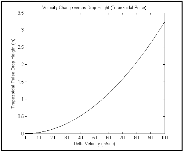
Figure description:
Velocity Change versus Drop Height (Trapezoidal Pulse
Velocity Change versus Drop Height (Trapezoidal Pulse
| Delta Velocity (in/sec) | Trapezoidal Pulse Drop Height (in) |
|---|---|
| 0 | 0.00 |
| 10 | 0.03 |
| 20 | 0.13 |
| 30 | 0.29 |
| 40 | 0.52 |
| 50 | 0.81 |
| 60 | 1.17 |
| 70 | 1.59 |
| 80 | 2.08 |
| 90 | 2.63 |
| 100 | 3.25 |
Notes: The data points are estimated based on the visual curve in the graph, which follows a quadratic relationship.
Figure 516.8-7. Fragility Shock Trapezoidal Pulse: velocity change versus drop height.
| Test | Peak Value1 (Am) G's | Nominal Duration2 (TD) (sec) |
|---|---|---|
| Fragility | 10-50 | TD = 2√2gh⁄Amg = 2√2h/g⁄Am |
Note 1: is dependent upon drop height "h." Typical range is provided (refer to paragraph 4.6.4). Note 2: "h" units: (in) and .
For a complex transient, there is no simple relationship between peak acceleration, pulse duration, and a change in velocity. It is assumed here that for a complex transient, velocity change is related to a significant difference between successive instantaneous peaks. (This can be determined with some effort by selecting positive and negative thresholds for which a few, e.g., five or fewer, positive and negative peaks alternate over suitably short periods of time.) In this case, change in velocity is not so much an instantaneous change upon impact, but may be a successive set of changes occurring at significant periods lower than those of acceleration. (Recall that velocity is a 1/(2лf) scaling of the acceleration frequency domain information.) For test materiel where a degree of precision is needed in specifying the level of input and correlation of the shock effects on the materiel with the level of input, simple base input SDOF modeling is suggested with subsequent integration of the equations of motion to determine the relative velocity and displacement. Simply scaling the peak acceleration level (in effect the square-root of the energy) of the pulse likewise scales the velocity change directly for a linear system. The same relationship between the variables holds, except now a "distribution" of velocity change in the complex transient must be considered as opposed to a single large velocity change as in the case of the trapezoidal pulse.
MIL-STD-810H
METHOD 516.8
Paragraph 4.6.4.c above implies that an analysis of the materiel has been completed prior to testing, that critical elements have been identified with their "stress thresholds," and that a failure model of the materiel relative to the shock input level has been developed. In addition, during the test, the "stress thresholds" of these critical elements can be monitored, and input to a failure model to predict failure at a given shock input level. In general, such input to the materiel produces large velocities and large changes in velocity. If the large velocity/velocity change exceeds that available on standard electrodynamic and/or servo-hydraulic test equipment, for this procedure the classical trapezoidal pulse may be used on properly calibrated drop machines. However, if the large velocity/velocity change is compatible with the capabilities of electrodynamic and/or servo-hydraulic test equipment, consider tailoring the shock according to a complex transient for application on the electrodynamic or servo-hydraulic test equipment. Using a trapezoidal pulse on electrodynamic and/or servo-hydraulic test equipment is acceptable (accounting for pre- and post-exciter positioning) if there are no available data providing shock input information that is tailorable to a complex transient. In summary, there is a single parameter (peak amplitude of the shock input) to define the fragility level holding the duration of the shock, , approximately constant. In the case of SRS synthesis, maximum velocity change is not as well defined, nor as easily controllable as for the classical trapezoidal pulse. Tailoring of the test is required when data are available, can be measured, or can be estimated from related data using accepted dynamic scaling techniques. An inherent assumption in the fragility test is that damage potential increases linearly with input shock level. If this is not the case, other test procedures may need to be used for establishing materiel fragility levels.
4.6.4.1 Test Controls – Fragility (Procedure III)
a. Specify the duration of the shock, , as it relates to the first fundamental mode of the materiel. Select a design drop height, h, based on measurement of the materiel's shipping environment, or from Transit Drop Tables 516.8-IX thru 516.8-XI as appropriate to the deployment environment when measured data are unavailable. (A design drop height is the height from which the materiel might be dropped in its shipping configuration and be expected to survive.) The maximum test item velocity change may then be determined by using the following relationship for 100% rebound:
where,
: maximum product velocity change () (summation of impact velocity and rebound velocity) h: design drop height in m (in) g: ()
The maximum test velocity change assumes 100 percent rebound. Programming materials, other than pneumatic springs, may have less than 100 percent rebound, so the maximum test velocity needs to be decreased accordingly. If the maximum test velocity specified is used for drop table shock machine programming materials other than pneumatic springs, the test is conservative (an over-test), and the maximum test item velocity is a bounding requirement.
- b. Set the shock machine to an acceleration level (Am) as determined based upon T D and ∆ V , well below the anticipated fragility level. If no damage occurs, increase Am incrementally (along with ∆ V ) while holding the pulse duration T constant until damage to the test item occurs. This will establish the materiel’s critical D acceleration fragility (or velocity change) level.
- c. Test levels used in this procedure represent the correlation of the best information currently available from research and experience. Use more applicable test level data if they become available (paragraph 6.1, reference g). In particular, if data are collected on a materiel drop and the SRS of the environment computed, a scaled version of the SRS could be used to establish the acceleration fragility level with respect to a measured environment on electrodynamic or servo-hydraulic test equipment, provided the displacement and velocity limitations of the test equipment are not exceeded. In addition to the maximax acceleration response spectra, compute the pseudo-velocity response spectra.
MIL-STD-810H
METHOD 516.8
4.6.4.2 Test Tolerances – Fragility (Procedure III)
It is assumed that the instrumentation noise in the measurements is low so that tolerances may be established. For complex transients from measured data, ensure test tolerances are consistent with the general guidelines provided in paragraph 4.2.2. For classical pulse testing, ensure the test tolerances specified in Figure 516.8-4, with respect to the information provided in Table 516.8-VIII, are satisfied.
4.6.4.3 Test Procedure – Fragility (Procedure III)
This test is designed to build up in severity as measured in peak acceleration or velocity change until a test item failure occurs, or a predetermined goal is reached. It may be necessary to switch axes between each shock event unless critical axes are determined prior to test. In general, all axes of importance will be tested at the same level before moving to another level. The order of test activity and the calibration requirements for each test setup should be clearly established in the test plan. It is also desirable to pre-select the steps in severity based on knowledge of the materiel item or the test environment, and document this in the test plan. Unless critical stress thresholds are analytically predicted and instrumentation used to track stress threshold buildup, there is no rational way to estimate the potential for stress threshold exceedance at the next shock input level. The following procedures, one for a classical pulse and the other for a complex transient, are written as if the test will be conducted in one axis alone. In cases where more test axes are required, modify the procedure accordingly.
- a. Classical Pulse. This part of the procedure assumes that the classical pulse approach is being used to establish the fragility level by increasing the drop height of the test item, thereby increasing the directly. The fragility level is given in terms of the measurement variable-peak acceleration of the classical pulse while holding the pulse duration as a function of the materiel modal characteristics a constant. In using this procedure, estimate the first mode mounted frequency of the materiel in order to specify the pulse duration .
- Step 1 Mount the calibration load to the test apparatus in a configuration similar to that of the actual test item. Use a fixture similar in configuration to the interface of the shock attenuation system (if any) that will support the materiel. The fixture should be as rigid as possible to prevent distortion of the shock pulse input to the test item.
Step 2 Perform calibration shocks until two consecutive shock applications to the calibration load reproduce the waveforms that are within the specified test tolerances. If response to the calibration shock is nonlinear with respect to shock input level, other test procedures may need to be applied to establish materiel fragility levels depending upon the extent of the nonlinearity prior to reaching the "stress threshold".
Step 3 Select an initial drop height low enough to assure that no damage will occur by selecting a fraction of the anticipated service drop height established from Transit Drop Tables 516.8-IX thru 516.8-XI. The maximum velocity change can be taken to be:
Where: : maximum test item velocity change, m/s (in/s) (assumes full resilient rebound of test item) h: drop height, m (in.) g: acceleration of gravity
Step 4 Mount the test item in the fixture. Perform an operational check and document the pre-test condition. If the test item operates satisfactorily, proceed to Step 5. If not, resolve the problems and repeat this step.
Step 5 Perform the shock test at the selected level, and examine the recorded data to assure the test is within tolerance.
Step 6 Visually examine and operationally check the test item to determine if damage has occurred. If the test item does not operate satisfactorily, follow the guidance in paragraph 4.3.2 for test item failure.
- Step 7 If it is required to determine the fragility of the test item in more than one axis, proceed to test the item (Steps 4-6) in the other axes (before changing the drop height).
Step 8 If the test item integrity is preserved, select the next drop height.
Step 9 Repeat Steps 4 through 8 until the test objectives have been met.
- Step 10 Perform a post shock operational test of the test item. See paragraph 5 for analysis of results. Document the results, including plots of the measured test response waveforms, and any pre- or post-shock operational anomalies.
- b. Synthesized Pulse. This part of the procedure assumes that the fragility level is some function of the peak acceleration level that correlates with a maximax acceleration SRS of a complex transient base input (because stress relates to velocity a peak pseudo-velocity level determined from a maximax pseudo-velocity SRS of a complex transient is preferable). For a complex transient specified in the time domain, this procedure generally uses the peak acceleration of the time history to define the fragility level.
- Step 1 Mount the calibration load to the test apparatus in a configuration similar to that of the actual test item. Use a fixture similar in configuration to the interface of the shock attenuation system (if any) that will support the materiel. The fixture should be as rigid as possible to prevent distortion of the shock pulse input to the test item.
- Step 2 Perform calibration shocks until two consecutive shock applications to the calibration load reproduce maximax acceleration SRS or pseudo-velocity SRS that are within the specified test tolerances. If response to the calibration shock is nonlinear with respect to shock input level, other test procedures along with simple modeling may need to be applied to establish materiel fragility levels, depending upon the extent of the nonlinearity prior to reaching the "stress threshold".
- Step 3 Select a peak maximax acceleration (or pseudo-velocity) SRS level low enough to assure no damage will occur.
- Step 4 Mount the test item in the fixture. Inspect and operationally test the item to document the pre-test condition. If the test item operates satisfactorily, proceed to Step 5. If not, resolve the problems and repeat this step.
- Step 5 Perform the shock test at the selected level, and examine the recorded data to assure the test maximax acceleration (or pseudo-velocity) SRS is within tolerance.
- Step 6 Visually examine and operationally check the test item to determine if damage has occurred. If so, follow the guidance in paragraph 4.3.2 for test item failure.
- Step 7 If it is required to determine the fragility of the test item in more than one axis, proceed to test the item in the other axes (before changing the peak maximax acceleration (or pseudo-velocity) SRS level).
- Step 8 If the test item integrity is preserved, select the next predetermined peak maximax acceleration (or pseudo-velocity) SRS level.
- Step 9 Repeat Steps 5 through 8 until the test objectives have been met.
- Step 10 Perform a post shock operational test of the test item. See paragraph 5 for analysis of results. Document the results, including plots of the measured test response waveforms and any pre- or post- shock operational anomalies.
4.6.5 Transit Drop (Procedure IV)
The intent of this test is to determine the structural and functional integrity of the materiel to a transit drop either outside or in its transit or combination case. In general, there is no instrumentation requirement for the test and measurement information is minimized, however, if measurements are made, the maximax acceleration SRS and the pseudo-velocity SRS will define the results of the test, along with the measurement amplitude time history.
MIL-STD-810H METHOD 516.8
4.6.5.1 Test Controls - Transit Drop (Procedure IV)
Test levels for this test are based on information provided in Tables 516.8-IX thru 516.8-XI. Test the item in the same configuration that is used in transportation, handling, or a combat situation. Toppling of the item following impact will occur in the field and, therefore, toppling of the test item following its initial impact should not be restrained as long as the test item does not leave the required drop surface. Levels for this test were set by considering how materiel in the field might commonly be dropped. Conduct all drops using a quick release hook, or drop tester. Use of a standardized impact surface is recommended for test repeatability because the surface configuration can influence test results. For most drop test requirements, steel plate on reinforced concrete is the default impact surface. The plate shall be homogenous material with a minimum thickness of 3 inches (76 mm) and Brinell hardness of 200 or greater. The plate shall be uniformly flat within commercial mill production standards, level within 2 degrees, and free of surface irregularities that may influence impact results. The concrete shall have a minimum compressive strength of 2500 psi (17 MPa), and be reinforced as required to prevent fracture during testing. In high velocity hazard classification drop scenarios (e.g. 40 ft) it is necessary for the concrete strength be 4000 psi with a minimum thickness of 24 inches. The steel plate shall be bonded and/or bolted to the concrete to create a uniform rigid structure without separation. The concrete foundation plus the impact plate mass shall be a minimum of 20 times the mass of the test item. The plate surface dimensions shall be sufficiently large to provide direct and secondary rotational impacts, and if possible rebound impacts. Guidance systems which do not reduce the impact velocity may be employed to ensure correct impact angle; however the guidance shall be eliminated at a sufficient height above the impact surface to allow unimpeded fall and rebound. Use of armor plate or similar composition steel plate is recommended to improve steel surface durability and prevent impact indentation and cuts. The impact surface shall be free from standing water, ice, or other material during testing. The most severe damage potential is impact with a non-yielding mass that absorbs minimal energy. Thus, use of a single monolithic impact mass is recommended to reduce energy transfer into the mass rather than the test item. The impact mass rigidity and energy transfer can be evaluated by measurement of the mass acceleration during testing.
Tables 516.8-IX thru 516.8-XI provide default drop conditions for transport from manufacturer to the end of its service life. Table 516.8-IX (Logistic Transit Drop Test) includes drop scenarios generally associated with non-tactical, logistical transport based on weight and test item dimensions. Table 516.8-X (Tactical Transport Drop Test) includes drop scenarios generally associated with tactical transport beyond the theatre storage area. As a default, the criteria for the tactical transport drop tests are to meet all performance requirements. For items that are incapable of meeting performance requirements, adjustments may be made to the drop height or configuration to accommodate the item performance limitations. If the drop conditions are modified, restrictions may be placed on the deployment of the item. Ensure an adequate test is performed and all deviations from this procedure are properly documented. Table 516.8-XI (Severe Tactical Transport Drop Test) includes severe drop scenarios, and the item is considered to have passed if it did not explode, burn, spread propellant or explosive material as a result of dropping, dragging or removal of the item for disposal. Other drop scenarios in the LCEP should be considered.
Realistic variations to the default values provided in Tables 516.8-IX thru 516.8-XI may be permitted when justified; e.g. large/complex systems in which specific handling considerations are identified in the LCEP may supersede the default levels provided.
Figure 516.8-8 illustrates the standard drop orientations as referenced in Tables 516.8-IX thru 516.8-XI. Figure 516.8-9 illustrates typical edge and corner drop configurations for large packages as discussed in Notes 2-4 of Table 516.8-IX.
MIL-STD-810H
METHOD 516.8
| Weight of Test Item & Case kg (lbs) | Largest Dimension cm (in.) | Notes | Height of Drop, h cm (in.) | Number of Drops |
|---|---|---|---|---|
| Under 45.4 (100) Man-packed or man-portable | Under 91 (36) | 122 (48) | Drop on each face, edge and corner; total of 26 drops5 | |
| 91 (36) & over | 76 (30) | |||
| 45.4–90.8 (100–200) inclusive | Under 91 | 76 (30) | Drop on each corner; total of eight drops | |
| 91 (36) & over | 61 (24) | |||
| 90.8–454 (200–1000) inclusive | Under 91 | 61 (24) | ||
| 91–152 (36–60) | 2 | 61 (24) | ||
| Over 152 (over 60) | 2 | 61 (24) | ||
| Over 454 (1000) | No limit | 3 4 | 46 (18) | Drop on each bottom edge. Drop on bottom face or skids; total of five drops |
- Note 1: Perform drops from a quick-release hook or drop tester. Orient the test item so that, upon impact, a line from the struck corner or edge to the center of gravity of the case and contents is perpendicular to the impact surface. The default drop surface is steel backed by concrete. Concrete or 5 cm (2 in) plywood backed by concrete may be selected if (a) a concrete or wood surface is representative of the most severe service conditions or (b) it can be shown that the compressive strength of the impact surface is greater than that of the test item impact point(s). Note that the shorter shock duration associated with the steel impact surface may not excite all test item resonant modes.
- Note 2: With the longest dimension parallel to the floor, support the transit, or combination case with the test item within, at the corner of one end by a block 13 cm (five inches) in height, and at the other corner or edge of the same end by a block 30 cm (12 inches) in height. Raise the opposite end of the case to the specified height at the lowest unsupported corner and allow it to fall freely.
- Note 3: While in the normal transit position, subject the case and contents to the edgewise drop test as follows (if the normal transit position is unknown, orient the case so the two longest dimensions are parallel to the floor):
Edgewise drop test: Support one edge of the base of the case on a sill 13-15 cm (five to six inches) in height. Raise the opposite edge to the specified height and allow it to fall freely. Apply the test once to each edge of the base of the case (total of four drops).
- Note 4: For shelters without shock attenuated skids, the drop height may be reduced to 15 cm (6 in) with a 10 cm (4 in) sill for edgewise drops.
- Note 5: If desired, divide the 26 drops among no more than five test items (see paragraph 4.6.5.1).
MIL-STD-810H
METHOD 516.8
| Scenario | Category | Impact Velocity (m/sec) | Drop Height1 (m) | Configuration | # Drops / Orientation 3,6 | Impact Surface | |
|---|---|---|---|---|---|---|---|
| Ship Transport | Storage and transport to theatre storage area, transport by ship | 5.4 (17.7 ft/sec) | 1.5m (5 ft) | Packaged6 | (minimum of 3) | Flat bottom and two faces.4 | Steel7,8 backed by concrete |
| Unpackaged Handling | Infantry and man- carried equipment | 5.4 (17.7 ft/sec) | 1.5m (5 ft) | Unpackaged | 5 | Steel7,8 backed by concrete | |
| Packaged Handling | Loading and offloading from side of transport vehicle - transport by truck, forklift, & helicopter | 6.4 (21 ft/sec) | 2.1m (7 ft) | Packaged6 | 5 | Flat bottom, two faces4 and two edges3 | Steel7,8 backed by concrete |
| Helicopter | Underslung load, quick release onto land or ship | 6.4 (21 ft/sec) | 2.1m (7 ft) | Packaged6 | 1 | Flat bottom | Steel7,8 backed by concrete |
| Parachute Drop2 | Low velocity drop | 8.7 (28.5 ft/sec) | 3.8m (12.6 ft) | Packaged with appropriate honeycomb or other shock absorbing system used in delivery | 1 | Flat bottom | Concrete |
| Parachute Drop | High velocity drop | 27.3 (90 ft/sec) | 38.1m (125 ft) | Concrete | |||
- Note 1: The test is not intended to encompass all credible accident conditions or severe mishandling conditions. Where the drop heights quoted are exceeded by those specified elsewhere in the table or for other phases of Service, the higher values should be substituted.
- Note 2: Drop heights are provided for simulated parachute drops. This test may not fully address certain effects that can occur during parachute drops in high wind conditions. Consider different drop height and angles of impact to address these issues. Drop from aircraft may be required for airdrop certification.
- Note 3: Sufficient assets are required to test in each of the orientations specified. Five standard drop orientations are listed in Table XII and illustrated in Figure 8. Consider other drop orientations if expected to have a greater damage potential. Expose each item to no more than 2 drops.
Note 4: For munitions, the two faces shall be the forward and aft ends of the munition.
Note 5: For munitions, the two edges shall be at 45 degrees on the forward and aft ends.
Note 6: Unpackaged if required by LCEP or Test Plan.
- Note 7: The default drop surface is steel backed by concrete. Concrete or 5 cm (2 in) plywood backed by concrete may be selected if (a) a concrete or wood surface is representative of the most severe service conditions or (b) it can be shown that the compressive strength of the impact surface is greater than that of the test item impact point(s). Note that the shorter shock duration associated with the steel impact surface may not excite all test item resonant modes.
- Note 8: A steel impact surface shall have a Brinell hardness of at least 200. For test items less than 454 kg (1000 lbs) the steel plate shall be at least 2.5 cm (1 in) thick, otherwise it shall be at least 7.6 cm (3 in) thick.
| Scenario | Category | Impact Velocity (m/sec) | Drop Height (m) | Configuration | # Drops / Orientation4,5 | |
|---|---|---|---|---|---|---|
| Helicopter | External Carriage on Helicopter | 6.4 (21 ft/sec) | 2.1m (7 ft) | Unpackaged | Flat Bottom, two faces² and two edges³ | |
| Military Land Vehicles | Includes weapons loading and off loading | 7.7 (25.3 ft/sec) | 3.05m (10 ft) | Unpackaged | 5 | |
| Aircraft | External Carriage on Fixed Wing Aircraft | 7.7 (25.3 ft/sec) | 3.05m (10 ft) | Unpackaged | ||
| Crane | Accidental Crane Drop | 15.5 (50.9 ft/sec) | 12.2m (40 ft) | Packaged¹ | ||
| Ship Transport | Shipboard Loading | 15.5 (50.9 ft/sec) | 12.2m (40 ft) | Packaged¹ | (minimum of 3) | Flat Bottom and two faces.² |
| Ship Aircraft Carrier | Shipboard Loading and Handling | 22.1 (72.5 ft/sec) | 25m (82 ft) | Packaged¹ | 5 | Flat Bottom, two faces² and two edges³ |
- Note 1: Unpackaged if required by LCEP or Test Plan.
- Note 2: For munitions, the two faces shall be the forward and aft ends of the munition.
- Note 3: For munitions, the two edges shall be at 45 degrees on the forward and aft ends.
- Note 4: Sufficient assets are required to test in each of the orientations specified. Five standard drop orientations are shown listed in Table 10 and illustrated in Figure 8. Other drop orientations should be considered if expected to have a greater damage potential. Each item should be exposed to no more than 2 drops.
Note 5: The default drop surface is steel backed by concrete. Concrete or 5 cm (2 in) plywood backed by concrete may be selected if (a) a concrete or wood surface is representative of the most severe service conditions or (b) it can be shown that the compressive strength of the impact surface is greater than that of the test item impact point(s). Note that the shorter shock duration associated with the steel impact surface may not excite all test item resonant modes.
| Drop | Rectangular Packages | Cylindrical Packages |
|---|---|---|
| 1 | Flat Bottom | Horizontal (Side 1) |
| 2 | Face 1: (Left End) | Face 1: (Fwd End/Top) |
| 3 | Face 2: (Right End) | Face 2: (Aft End/Bottom) |
| 4 | Edge 1: (Bottom Right End Edge) | Edge 1: (Aft End Bottom Edge (45 Deg)) |
| 5 | Edge 2: (Top Left Edge) | Edge 2: Fwd End Top Edge (45 Deg)) |
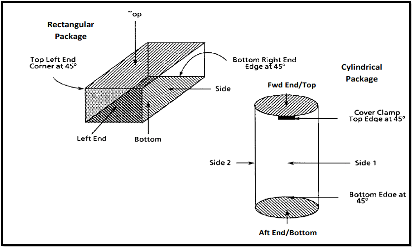
Figure description:
Figure 516.8-8: Standard drop orientations for rectangular and cylindrical packages.
Rectangular Package Orientations:
- Faces: Top, Bottom, Side, Left End
- Edges/Corners:
- Top Left End Corner at 45°
- Bottom Right End Edge at 45°
Cylindrical Package Orientations:
- Ends: Fwd End/Top, Aft End/Bottom
- Sides: Side 1, Side 2
- Edges:
- Cover Clamp Top Edge at 45°
- Bottom Edge at 45°
Figure 516.8-8. Standard drop orientations for rectangular and cylindrical packages.
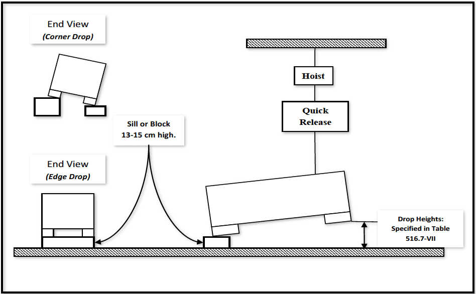
Figure description:
Figure 516.8-9: Illustration of edge drop configuration
- Test Components:
- Hoist and Quick Release: Mechanism used to lift and release the test article.
- Sill or Block: Support used for one side of the article, measuring 13-15 cm high.
- Test Article: Shown in tilted positions for drop testing.
- Configurations Illustrated:
- Edge Drop: Main side view and end view showing the article resting on a block on one side.
- Corner Drop: End view showing the article tilted and supported at a corner.
- Key Parameters:
- Sill/Block Height: 13-15 cm.
- Drop Heights: Defined by Table 516.7-VII.
Figure 516.8-9. Illustration of edge drop configuration (corner drop end view is also illustrated).
4.6.5.2 Test Tolerances - Transit Drop (Procedure IV)
Ensure the test height of drop is within 2.5 percent of the height of drop as specified in Tables 516.8-IX through 516.8- XI.
4.6.5.3 Test Procedure - Transit Drop (Procedure IV)
- Step 1 After performing a visual inspection and operational check for baseline data, install the test item in its transit or combination case as prepared for field use (if measurement information is to be obtained, install and calibrate such instrumentation in this Step). If the test item operates satisfactorily, proceed to Step 2. If not, resolve the problems and repeat this step.
- Step 2 From paragraph 4.6.5.1 and Tables 516.8-IX-516.8-XI, determine the height of the drops to be performed, drop orientation, the number of drops per test item, and the drop surface.
- Step 3 Perform the required drops using the apparatus and requirements of paragraphs 4.6.5 and 4.6.5.1 and Tables 516.8-IX through 516.8-XI notes. Recommend visually and/or operationally checking the test item periodically during the drop test to simplify any follow-on evaluation that may be required. If any degradation is noted, see paragraph 4.3.2.
- Step 4 Document the impact point or surface for each drop and any obvious damage.
- Step 5 Following completion of the required drops, visually examine the test item(s), and document the results.
- Step 6 Conduct an operational checkout in accordance with the approved test plan. See paragraph 5 for analysis of results.
- Step 7 Document the results for comparison with data obtained in Step 1, above.
MIL-STD-810H
METHOD 516.8
4.6.6 Crash Hazard Shock (Procedure V)
The intent of this procedure is to disclose structural failures of materiel or mounts for materiel in air or ground vehicles that may present a hazard to personnel or other materiel if the materiel breaks loose from its mount during or after a vehicle crash. This test procedure is intended to verify that materiel mounting and/or restraining devices will not fail, and that sub-elements are not ejected during crash situations. Attach the test item to its shock fixture by its in-service mounting or tie-downs.
For materiel weighing less than 227 g (8 ounces) it may be permissible to omit the crash hazard test if it is determined that personnel expected to be in the vicinity of the test article are equipped with sufficient Personal Protective Equipment -PPE (i.e., helmets with visors) such that risk of significant bodily injury is determined to be highly unlikely. In addition to the item's mass, assess overall material properties and geometry when considering omitting Procedure V. Final decisions in such cases are left to the discretion of the responsible safety authority, and based upon the case-specific hazard analysis.
4.6.6.1 Test Controls - Crash Hazard Shock (Procedure V)
Use Table 516.8-III and Figure 516.8-2 as the test spectrum and effective durations. If shock spectrum analysis capabilities are not available, a classical pulse may be used as an alternative to a complex transient waveform developed from the SRS in Figure 516.8-2. Table 516.8-XIII provides the parameters for the default terminal peak sawtooth. An aircraft crash level of 40 G's is based on the assumption that, during a survivable crash, localized G levels can approach 40 G's. Ground transportation vehicles are designed with a higher safety factor and, therefore, must sustain a much higher G level with correspondingly higher specified test levels.
Table 516.8-XIII. Terminal peak sawtooth default test parameters for
Procedure V – Crash Hazard (refer to Figure 516.8-3).
Test: Minimum Peak Value and Pulse Duration: Am (G-Pk) & TD(ms): Flight Vehicle Materiel1: Ground Materiel1:
Procedure V -Crash Hazard: Flight Vehicle Materiel1: 40 G Flight Vehicle Materiel1: 11 ms Ground Materiel1: 75 G Ground Materiel1: 6 ms
Note 1. For materiel that is shock-mounted or weighing more than 136 kg (300 lbs), an 11 ms half-sine pulse of such amplitude that yields an equivalent velocity to the default terminal peak sawtooth may be employed.
4.6.6.2 Test Tolerances - Crash Hazard Shock (Procedure V)
For complex waveform replication based on SRS, ensure the test tolerances are within those specified for the SRS in paragraph 4.2.2. For the classical terminal peak sawtooth and half-sine options defined in Table 516.8-XIII, ensure the waveform is within the tolerances specified in Figures 516.8-3 and 5.
4.6.6.3 Test Procedure - Crash Hazard Shock (Procedure V)
- Step 1 Secure the test item mount to the shock apparatus by its in-service mounting configuration. Use a test item that is dynamically similar to the materiel, or a mechanically equivalent mockup. If a mockup is used, it will represent the same hazard potential, mass, center of mass, and mass moments about the attachment points as the materiel being simulated. (If measurement information is to be collected, mount and calibrate the instrumentation.)
- Step 2 Perform two shocks in each direction (as determined in paragraph 2.3.3) along three orthogonal axes of the test item for a maximum of 12 shocks.
Step 3 Perform a physical inspection of the test setup. Operation of the test item is not required.
- Step 4 Document the results of the physical inspection, including an assessment of potential hazards created by either materiel breakage or structural deformation, or both. Process any measurement data according to the maximax acceleration SRS or the pseudovelocity SRS.
4.6.7 Bench Handling (Procedure VI)
The intent of this test is to determine the ability of materiel to withstand the usual level of shock associated with typical bench maintenance or repair. Use this test for any materiel that may experience bench or bench-type maintenance. This test considers both the structural and functional integrity of the materiel.
4.6.7.1 Test Controls - Bench Handling (Procedure VI)
Ensure the test item is a fully functional representative of the materiel. Raise the test item at one edge 100 mm (4 in.) above a solid wooden bench top, or until the chassis forms an angle of 45° with the bench top or until point of balance is reached, whichever is less. (The bench top must be at least 4.25 cm (1.675 inches) thick.) Perform a series of drops in accordance with specifications. The heights used during this test are defined by examining the typical drops that are commonly made by bench technicians and assembly line personnel.
4.6.7.2 Test Tolerances - Bench Handling (Procedure VI)
Ensure the test height of drop is within 2.5 percent of the height of drop as specified in paragraph 4.6.7.1.
4.6.7.3 Test Procedure - Bench Handling (Procedure VI)
- Step 1 Following an operational and physical checkout, configure the item as it would be for servicing, e.g., with the chassis and front panel assembly removed from its enclosure. If the test item operates satisfactorily, proceed to Step 2. If not, resolve the problems and repeat this Step. Position the test item as it would be for servicing. Generally, the test item will be non-operational during the test.
- Step 2 Using one edge as a pivot, lift the opposite edge of the chassis until one of the following conditions occurs (whichever occurs first).
- a. The lifted edge of the chassis has been raised 100 mm (4 in.) above the horizontal bench top.
- b. The chassis forms an angle of 45° with the horizontal bench top.
- c. The lifted edge of the chassis is just below the point of perfect balance.
Let the chassis drop back freely to the horizontal bench top. Repeat using other practical edges of the same horizontal face as pivot points, for a total of four drops.
- Step 3 Repeat Step 2 with the test item resting on other faces until it has been dropped for a total of four times on each face on which the test item could be placed practically during servicing.
Step 4 Visually inspect the test item.
Step 5 Document the results.
- Step 6 Operate the test item in accordance with the approved test plan. See paragraph 5 for analysis of results.
Step 7 Document the results for comparison with data obtained in Step 1, above.
4.6.8 Pendulum Impact (Procedure VII)
The test item (large shipping container) may consist of a box, case, crate or other container constructed of wood, metal, or other material, or any combination of these for which ordinary box tests are not considered practical or adequate. Unless otherwise specified, large containers are those that measure more than 152cm (60 in.) on any edge or diameter, or those when loaded have gross weights in excess of 70kg (154 lbs).
4.6.8.1 Test Controls - Pendulum Impact (Procedure VII)
- a. The pendulum impact tester consists of a platform suspended from a height at least 5m (16.4 ft) above the floor by four or more ropes, chains, or cables; and a bumper comprised of a flat, rigid concrete or masonry wall, or other equally unyielding flat barrier. The bumper is at least 46cm (18.1 in) high; wide enough to make full contact with the container end, and has sufficient mass to resist the impacts without displacement. The impact surface is oriented perpendicular to the line of swing of the platform. The platform is large enough to support the container or pack, and when hanging free, has its top surface approximately 23cm (9.1 in) above the floor, and its leading edge at least 8cm (3.1 in) from the surface of the bumper. The suspension
chains are vertical and parallel so that when the platform is pulled straight back, it will rise uniformly but remain at all times horizontal and parallel to the floor (see Figure 516.8-10).
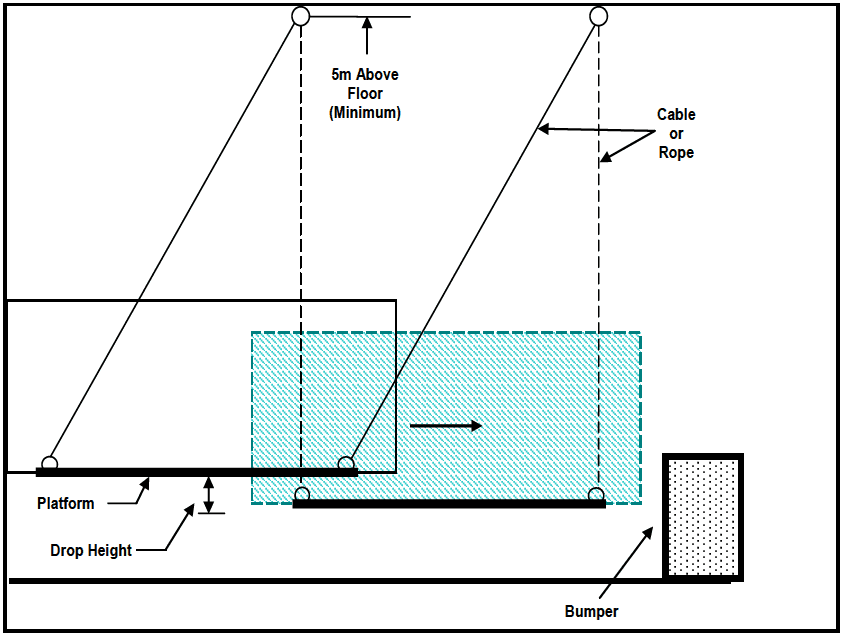
Figure description:
Key Entities and Information:
- Platform: A horizontal surface suspended by parallel cables or ropes.
- Cable or Rope: Support lines connecting the platform to overhead mounting points.
- Suspension Height: Mounting points are located a minimum of 5m above the floor.
- Drop Height: The vertical distance between the platform's raised starting position and its horizontal position at impact.
- Bumper: A stationary impact block positioned at the end of the platform's swing path.
- Mechanism: The platform is pulled back and released, swinging forward while remaining horizontal until it strikes the bumper.
Figure 516.8-10. Pendulum impact test
- b. The drop height shall be determined for the required horizontal impact velocity based on the transfer of potential to kinetic energy (h = v²/2g). Unless otherwise specified, the vertical height is a drop of 23 cm (9 in.) that results in a velocity of 2.13m/sec (7 ft/sec) at impact.
- c. Load the test item (container) with the interior packing and the actual contents for which it was designed. If use of the actual contents is not practical, a dummy load may be substituted to simulate such contents in weight, shape, and position in the container. Block and brace the contents, or dummy load, and cushion them in place as for shipment. When the pendulum impact test is performed to evaluate the protection provided for the contents, the rigidity of a dummy load should closely approximate that of the actual contents for which the pack was designed.
4.6.8.2 Test Tolerances - Pendulum Impact (Procedure VII)
Ensure the vertical drop height is within 2.5 percent of the required height.
4.6.8.3 Test Procedure - Pendulum Impact (Procedure VII)
- Step 1 If required, perform a pretest operational checkout in accordance with the test plan. Install accelerometers and other sensors on the test item, as required.
- Step 2 Place the test item on the platform with the surface that is to be impacted projecting beyond the front end of the platform so that the specimen just touches the vertical surface of the bumper.
- Step 3 Pull back the platform so that the center of gravity of the pack is raised to the prescribed height, and then release it to swing freely so that the surface of the container impacts against the bumper. Unless
MIL-STD-810H
METHOD 516.8
otherwise specified, the vertical height is a drop of 23cm (9 in.) that results in a velocity of 2.13m/sec (7 ft/sec) at impact.
- Step 4 Examine the test item and record obvious damage. If the container is undamaged, rotate it 180 degrees and repeat Step 3. When the test is conducted to determine satisfactory performance of a container or pack, and unless otherwise specified, subject each test item to one impact to each side and each end that has a horizontal dimension of less than 3m (9.8 ft).
- Step 5 Record any changes or breaks in the container, such as apparent racking, nail pull, or broken parts, and their locations. Carefully examine the packing (blocks, braces, cushions, or other devices) and the contents, and record their condition. If required, perform a post-test operational checkout in accordance with the test plan. See paragraph 5 for analysis of results.
4.6.9 Catapult Launch/Arrested Landing (Procedure VIII)
The intent of this test is to verify the functionality and structural integrity of materiel mounted in or on fixed wing aircraft that are subject to catapult launches and arrested landings.
4.6.9.1 Test Controls - Catapult Launch/Arrested Landing (Procedure VIII)
- a. Measured Data Not Available. Whenever possible, derive the test conditions from measured data on applicable carrying aircraft (see Part One, paragraph 5.6, as well as the tasks at the end of Part One in Annex A for information on the use of field/fleet data), since shock responses can be affected by local influences such as wing and fuselage bending modes, pylon interfaces, and structural damping. While the pulse amplitudes associated with this environment are generally low, the long periods of application and high frequency of occurrence have the potential to cause significant dynamic and/or low cycle fatigue damage in improperly designed materiel. A typical aircraft may fly as many as 200 sorties per year, of which more than two-thirds involve catapult launches and arrested landings. However, for laboratory test purposes, 30 simulated catapult/arrested landing events in each of two axes (longitudinal and vertical) should provide confidence that the majority of significant defects will be identified for remedial action. If acceptable field- measured data are not available, the following guidance is offered in which sinusoidal burst is used to simulate each catapult or launch event. This time history has been simplified to a constant amplitude sine burst of 2-second duration for simulation at the selected materiel frequency (usually the first fundamental mode of the loaded aircraft wing). For testing purposes, it is permissible to reduce the maximum amplitude in the horizontal direction to 75 percent of that in the vertical direction.
- (1) Wave shape: damped sine wave.
- (2) Wave frequency: determined by structural analysis of the specific aircraft and frequency of the fundamental mode.
- (3) Burst amplitude: determined by structural analysis of the specific aircraft, the frequency of the fundamental mode and the location of the materiel relative to the shape of the fundamental mode.
- (4) Wave damping (quality factor): Q = 20.
- (5) Axis: vertical, horizontal, longitudinal.
- (6) Number of bursts: determined by the specific application (for example, 30 bursts, each followed by a 10 second rest period).
- b. Measured Data Available. If acceptable field measured data are available, the following guidance is offered in which the catapult event is simulated by two shocks separated by a transient vibration, and the arrested landing event by one shock followed by transient vibration. The catapult launch/arrested landing shock environment differs from other typical shock events in that it is a transient periodic vibration (roughly sinusoidal) at a relatively low frequency determined by aircraft mass and landing gear damping characteristics. Typical catapult launch shock time histories are shown in Figure 516.8-11. These data represent measured acceleration response in the vertical, horizontal and longitudinal directions of a store component mounted on the pylon of a platform. The data are DC coupled and low pass filtered at 70 Hz. All three time histories demonstrate an initial transient, followed by a transient vibration (nearly two seconds long), and concluded by a final transient. The longitudinal axis provides a profile of the DC catapult acceleration that, in general, will not be important for testing purposes, and can be removed by high pass
filtering the time history at a frequency less than 10 percent of the lowest significant frequency in the maximax acceleration SRS. Procedures for accomplishing this filtering may necessarily be iterative (unless Fourier transform information is used) with high pass filtering beginning at a comparatively high frequency, and decreasing until the most significant SRS low frequency is identified. In general, catapult acceleration response will display two shock events corresponding to initial catapult load application to the aircraft and catapult release from the aircraft separated by an oscillatory acceleration. Both the initial and the final shock events have a distinct oscillatory nature. It is essential that this test be run as a series of two shock transients separated by a two second period of time in which transient vibration may be input. Typical arrested landing shock time histories are shown on Figure 516.8-12. These data represent measured acceleration response in the vertical, horizontal and longitudinal directions of a store component mounted on the pylon of a platform. The data are DC coupled and low pass filtered at 70 Hz. All three time histories demonstrate an initial transient, followed by a transient vibration (nearly three seconds long). It is clear that the longitudinal time history has a comparatively large DC component that may be filtered out for test specification development. The term “transient vibration” is introduced here because of the duration of the event being not typical of a shock event.
NOTE: Transient Vibrations. For precise laboratory simulation, Procedure VIII may require consideration of the concept of a transient vibration in processing and replication of the form of time history from measured data. For long duration transient environments (durations on the order of one second or more), it may be useful to process the response time history by estimating the envelope function, a(t), and proceeding to compute a maximax Autospectral Density Estimate (ASD), assuming short portions of the response time history behave in the same manner as stationary random data. Estimation of this form falls under the category of nonstationary time history processing and will not be considered further in this Method. For a precise definition of transient vibration, see Part One, Annex D. The importance of the transient vibration phenomenon is that (1) it has the form of a shock (short duration and substantial time varying amplitude), (2) it can be mathematically modeled in a precise way, and (3) it can be used in stochastic simulation of certain shock environments. In general, shocks have their significant energy in a shorter time frame than transient vibrations, while transient vibrations allow for time history enveloping functions other than the exponential envelope form often times displayed in shocks as a result of resonant response decay to an impact.
BULKHEAD VERTICAL 5.00 G -5.00 0.00 5 00
BULKHEAD HORIZONTAL 5.00 G -5.00 0.00 5.00
BULKHEAD LONGITUDINAL 10.00 G -10.00 0.00 5 00
Time (seconds)
Amplitude (g's)
Figure 516.8-11. Sample measured store three axis catapult launch component response acceleration time histories.
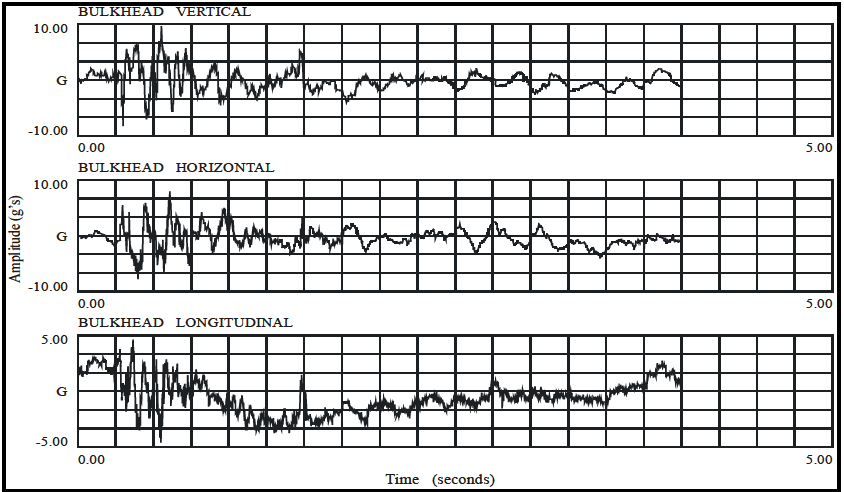
Figure description:
Vibration Amplitude vs Time Vibration Measurements for Bulkhead (Vertical, Horizontal, Longitudinal
BULKHEAD VERTICAL
Annotations
- G (Zero Line (horizontal_line - position: y = 0.00))
| Time (seconds) | Amplitude (G) |
|---|---|
| 0.00 | 0.00 |
| 0.15 | 2.50 |
| 0.25 | -2.00 |
| 0.35 | 6.00 |
| 0.45 | -8.00 |
| 0.55 | 9.00 |
| 0.65 | -9.50 |
| 0.75 | 5.00 |
| 0.85 | -8.50 |
| 0.95 | 10.00 |
| 1.10 | -9.00 |
| 1.25 | 4.00 |
| 1.50 | -3.00 |
| 1.75 | 7.50 |
| 2.00 | -1.00 |
| 2.25 | -4.00 |
| 2.50 | 1.50 |
| 2.75 | -2.50 |
| 3.00 | 2.00 |
| 3.25 | -1.50 |
| 3.50 | 0.50 |
| 3.75 | 2.50 |
| 4.00 | -0.50 |
BULKHEAD HORIZONTAL
Annotations
- G (Zero Line (horizontal_line - position: y = 0.00))
| Time (seconds) | Amplitude (G) |
|---|---|
| 0.00 | 0.00 |
| 0.15 | 1.50 |
| 0.25 | -3.00 |
| 0.35 | 5.50 |
| 0.45 | -7.50 |
| 0.55 | 6.50 |
| 0.65 | -10.00 |
| 0.75 | 8.00 |
| 0.85 | -6.50 |
| 0.95 | 9.00 |
| 1.10 | -5.00 |
| 1.25 | 4.50 |
| 1.50 | -2.50 |
| 1.75 | 6.50 |
| 2.00 | -2.00 |
| 2.25 | -4.50 |
| 2.50 | 3.50 |
| 2.75 | -3.50 |
| 3.00 | 0.50 |
| 3.25 | -4.00 |
| 3.50 | -1.50 |
| 3.75 | 0.50 |
| 4.00 | -1.00 |
BULKHEAD LONGITUDINAL
Annotations
- G (Zero Line (horizontal_line - position: y = 0.00))
| Time (seconds) | Amplitude (G) |
|---|---|
| 0.00 | 0.00 |
| 0.15 | 2.00 |
| 0.25 | 2.50 |
| 0.35 | 4.50 |
| 0.45 | -3.50 |
| 0.55 | 5.00 |
| 0.65 | -4.50 |
| 0.75 | 3.00 |
| 0.85 | -4.00 |
| 0.95 | 2.50 |
| 1.10 | -3.50 |
| 1.25 | -2.00 |
| 1.50 | -4.00 |
| 1.75 | -3.50 |
| 2.00 | -4.50 |
| 2.25 | -3.00 |
| 2.50 | -2.00 |
| 2.75 | -2.50 |
| 3.00 | -0.50 |
| 3.25 | -1.50 |
| 3.50 | 0.50 |
| 3.75 | 2.50 |
| 4.00 | 0.50 |
Notes: The plots display high-frequency vibration data over a 5-second interval. The signal in each chart terminates just before the 4.25-second mark. The vertical and horizontal components share a Y-axis scale of -10.00 to 10.00 G, while the longitudinal component uses a scale of -5.00 to 5.00 G.
Figure 516.8-12. Sample measured store three axis arrested landing component response acceleration time histories.
4.6.9.2 Test Tolerances - Catapult Launch/Arrested Landing (Procedure VIII)
For cases in which measured data are not available and waveforms are generated from dynamic analysis of the configuration, ensure the waveform tolerances are within the time history test tolerances specified for waveforms in paragraph 4.2.2. For cases in which measured data are available, ensure the SRS for the test response is within the SRS tolerances specified in paragraph 4.2.2. For transient vibration, ensure the waveform peaks and valleys are within the tolerances given for waveforms in paragraph 4.2.2 or as provided in the test specification.
4.6.9.3 Test Procedure - Catapult Launch/Arrested Landing (Procedure VIII)
- Step 1 Mount the test item to its shock/vibration fixture on the shock device for the first test axis.
- Step 2 Attach instrumentation as required in the approved test plan.
- Step 3 Conduct an operational checkout and visual examination in accordance with the approved test plan. If the test item operates satisfactorily, proceed to Step 4. If not, resolve the problems and repeat this step.
- Step 4a If no measured field data are available, apply short transient sine waves of several cycles to the test item in the first test axis. (Each short transient sine wave of several cycles represents a single catapult or arrested landing event.) Follow each burst by a rest period to prevent unrepresentative effects. Operate the test item in its appropriate operational mode while bursts are applied. If the test item fails to operate as intended, follow the guidance in paragraph 4.3.2 for test item failure.
- Step 4b If measured field data are available, either apply the measured response data under exciter system time waveform control (see Method 525.2), or process the catapult as two shocks separated by a transient vibration, and the arrested landing as a shock followed by a transient vibration. Operate the test item in its appropriate operational mode while bursts are applied. If the test item fails to operate as intended, follow the guidance in paragraph 4.3.2 for test item failure.
- Step 5 If the test item has not malfunctioned during testing, conduct an operational checkout and visual examination in accordance with the approved test plan. If a failure has occurred, it may be desirable to perform a thorough visual examination before proceeding with the operational checkout to avoid initiating additional hardware damage. When a failure occurs, consider the nature of the failure and corrective action, along with the purpose of the test (engineering information or contractual
compliance) in determining whether to restart the test or to continue from the point of interruption. If the test item does not operate satisfactorily, follow the guidance in paragraph 4.3.2 for test item failure.
Step 6 Repeat Steps 1 through 5 for the second test axis.
Step 7 Document the test results including amplitude time history plots, and notes of any test item operational or structural degradation. See paragraph 5 for analysis of results.