| PROCESSING | A-1 |
| 1.1 | MEASUREMENT SYSTEM AND SIGNAL CONDITIONING PARAMETERS | A-1 |
| 1.2 | MEASUREMENT SHOCK IDENTIFICATION | A-3 |
| 1.3 | EFFECTIVE SHOCK DURATION FOR NON-CLASSICAL SHOCKS | A-4 |
| 1.3.1 | CALCULATION OF Te | A-6 |
| 1.3.2 | CALCULATION OF TE | A-6 |
| 1.3.3 | IMPLEMENTATION CONSIDERATIONS | A-7 |
| 1.4 | SHOCK RESPONSE SPECTRUM | A-7 |
| 1.4.1 | PROCESSING GUIDELINES | A-7 |
| 1.4.2 | PROCESSING EXAMPLE | A-10 |
| 1.5 | FREQUENCY DOMAIN IDENTIFICATION ENERGY SPECTRAL DENSITY (ESD) | A-11 |
| 1.6 | SINGLE EVENT / MULTIPLE CHANNEL MEASUREMENT PROCESSING GUIDELINES | A-11 |
| 1.7 | MEASUREMENT PROBABILISTIC / STATISTICAL SUMMARY | A-11 |
| 1.8 | OTHER PROCESSING | A-12 |
ANNEX A FIGURES
| FIGURE 516.8A-1. | a. FILTER ATTENUATION | A-1 |
| FIGURE 516.8A-1. | b. ILLUSTRATION OF SAMPLING RATES AND OUT OF BAND "FOLD OVER" FREQUENCIES FOR DATA ACQUISITION SYSTEMS | A-3 |
| FIGURE 516.8A-2. | EXAMPLE ACCELERATION TIME HISTORY. | A-4 |
| FIGURE 516.8A-3. | EXAMPLE SIMPLE SHOCK TIME HISTORY WITH SEGMENT IDENTIFICATION | A-5 |
| FIGURE 516.8A-4. | MAXIMAX PSEUDO-VELOCITY SRS ESTIMATES FOR SHOCK AND NOISE FLOOR SEGMENTS | A-8 |
MIL-STD-810H
METHOD 516.8
CONTENTS - Continued
| Paragraph | Page |
|---|---|
| FIGURE 516.8A-5. SHOCK MAXIMUM AND MINIMUM PSEUDO-VELOCITY SRS ESTIMATES | .A-9 |
| FIGURE 516.8A-6. SHOCK MAXIMUM AND MINIMUM ACCELERATION SRS ESTIMATES | .A-10 |
| FIGURE 516.8A-7. MAXIMAX ACCELERATION SRS ESTIMATES FOR SHOCK AND NOISE FLOOR SEGMENTS | A-11 |
METHOD
516.8-1 SCOPE
516.8-1 SINGLE SHOCK EVENT MEASUREMENT SYSTEM CHARACTERIZATION AND BASIC PROCESSING
The following paragraphs discuss basic measurement system acquisition characteristics, followed by a discussion on the correct identification of the parts of a measured shock (in particular the duration of a shock). Information in Annex A is essential for the processing of measured data for a laboratory test specification.
516.8-1 INTRODUCTION
This Annex provides additional guidelines for shock time history assessment including validation, i.e., to detect any measurement system anomalies that would invalidate the measurement. For massive field shock measurement programs where time and budget constraints do not allow validation of individual shocks, at least one shock time history from each measurement channel needs to be individually validated, and careful examination of the time history for each subsequent shock from the measurement channel be examined for gross anomalies. Consistency relative to the test specification for processed information is acceptable as long as any inconsistency is investigated under shock time history validation. For example, the Normal Tolerance Limit (Annex C) when properly applied should be used only for collections of SRS estimates that have a similar shape; otherwise the variance is inflated beyond what might exist for field measured data under repeated experimental measurements.
516.8-1 SCOPE
1.1 Purpose
Shock tests are performed to:
- a. Provide a degree of confidence that materiel can physically and functionally withstand the shocks encountered in handling, transportation, and service environments. This may include an assessment of the overall materiel system integrity for safety purposes in any one or all of the handling, transportation, and service environments.
- b. Determine the materiel's fragility level, in order that packaging, stowage, or mounting configurations may be designed to protect the materiel's physical and functional integrity.
- c. Test the strength of devices that attach materiel to platforms that may be involved in a crash situation and verify that the material itself does not create a hazard or that parts of the materiel are not ejected during a crash situation.
516.8-1.1 Measurement System and Signal Conditioning Parameters
The data recording instrumentation shall have flat frequency response to the maximum frequency of interest ( ). If is not specified, a default value of 10 KHz is recommended for acquisition at each measurement location. Defining as the 3dB half-power point cut-off frequency of the low-pass analog anti-alias filter, is implied to maintain flat frequency response. The digitizing rate must be at least 2.5 times the filtering frequency . Note that when measurements of peak amplitude are used to qualify the shock level, a sample rate of at least 10 times the filtering frequency (100 thousand samples per second for the default case) is required. For SRS considerations a measurement shock should be acquired at 10 times the filtering frequency or resampled to 10 times the filtering frequency.
It is imperative that a responsibly designed signal conditioning system be employed to reject possibility of any aliasing. Analog anti-alias filters must be in place before the digitizing portion of the signal conditioning system. The selected anti-alias filtering must have an amplitude attenuation of 50 dB or greater, and a pass band flatness within one dB across the frequency bandwidth of interest for the measurement (see Figure 516.8-1a). Subsequent re-sampling for either up-sampling (interpolation) or down-sampling (decimation) must be in accordance with standard practices and consistent with the analog anti-alias configuration.).
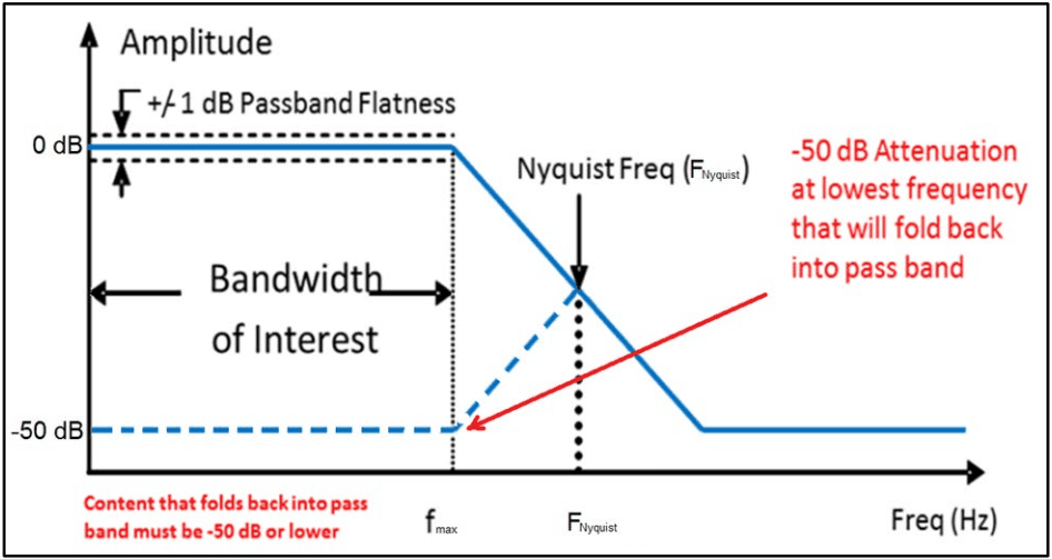
Figure description:
Anti-Aliasing Filter Characteristics and Requirements Diagram均衡器特性与要求图示表(英)
Amplitude vs Frequency
Legend
- Filter Response — color: blue; symbol: Solid line
- Aliased Fold-back — color: blue; symbol: Dashed line
Annotations
- +/- 1 dB Passband Flatness (text_label - position: y = 0 dB)
- Bandwidth of Interest (horizontal_range - position: x = 0 to f_max)
- Nyquist Freq (F_Nyquist (vertical_line - position: x = F_Nyquist))
- -50 dB Attenuation at lowest frequency that will fold back into pass band (text_label - position: x = 2 * F_Nyquist - f_max, y = -50 dB)
- Content that folds back into pass band must be -50 dB or lower (text_label - position: x < f_max, y = -50 dB)
| Frequency (Hz) | Filter Response (dB) | Aliased Fold-back (dB) |
|---|---|---|
| 0 | 0 | -50 |
| f_max | 0 | -50 |
| F_Nyquist | -25 | -25 |
| 2 * F_Nyquist - f_max | -50 | null |
| f_end | -50 | null |
Figure 516.8A-1a. Filter attenuation (conceptual, not filter specific).
The end to end alias rejection of the final digitized output must be shown to meet the requirements in Figure 516.8 A-1a. The anti-alias characteristics must provide an attenuation of 50 dB or greater for frequencies that will fold back into the bandwidth of interest (passband). Generally, for validly acquired digital shock time history data spectral data including SRS plots are only presented for frequencies within the passband (up to ). However, this restriction is
MIL-STD-810H
METHOD
516.8-1.1 Purpose
This Annex provides information relative to the statistical and probabilistic characterization of a set of data for the purpose of defining an “upper limit” on the data set. Such an upper limit may be subsequently used for an enveloping procedure for specification development (this Annex provides no guidance on “enveloping procedures,” where an “enveloping procedure” is defined as a procedure providing polynomial interpolation of spectral information for break point definition used directly in exciter control). Although limit estimates defined below may be applicable over a range of different independent variables it will be assumed for convenience that the independent variable is labeled “frequency”. (For other independent variables, e.g., time, serial correlation in the estimates may need to be accounted for in establishing limits.) It is assumed that input is empirical and representative of one of more random processes with unknown probabilistic specification (i.e., if the probabilistic structure of the random processes is known, statistical considerations contained herein would not be pertinent.)
1.2 Application
Use this Method to evaluate the physical and functional performance of materiel likely to be exposed to mechanically induced shocks in its lifetime. Such mechanical shock environments are generally limited to a frequency range not to exceed 10,000 Hz, and a duration of not more than 1.0 second. (In most cases of mechanical shock, the significant materiel response frequencies will not exceed 4,000 Hz, and the duration of materiel response will not exceed 0.1 second.)
516.8-1.2 Measurement Shock Identification
A “simple shock” is being addressed in this Method (excluding Procedure VIII and the example of a complex shock provided in Annex B), i.e., the impulse force input defines a single “event” arising from a characteristic phenomenon. A “simple shock” is defined by a measurement, e.g., acceleration, with three characteristic regions:
- a. An initial low amplitude stationary random measurement termed the measurement system noise floor.
- b. A series of erratic high amplitude decaying measurement amplitudes termed the shock.
- c. A comparatively low level stationary measurement at or just above the instrumentation noise floor termed the post-shock noise floor.
NOTE: If periodic components or non-Gaussian behavior are present in the measurement system noise floor, the signal conditioning system needs to be examined. If periodic components are present in the post-shock noise floor but the general amplitude is relatively stationary, it is indicative of mounting/materiel resonance response. A trained analyst needs to decide the importance of such resonance information in a laboratory test specification. This decision should be based upon the lowest mounted fundamental frequency of the materiel. In general, shock information should not be unduly extended in order to accommodate the full extent of the resonant “ringing” behavior.
It is always imperative that the data be carefully analyzed to ensure the measurement is free of corruption, and the nature of the event is physically well grounded. This subject is discussed in greater detail in Annex B.
MIL-STD-810H METHOD
516.8-1.2 Application
Information in this Annex is generally applicable to two or more frequency domain estimates that are either predicted based on given information, or on time domain measurements processed in the frequency domain according to an appropriate technique, e.g., for stationary random vibration, the processing would be an ASD; for a very short transient the processing could be an SRS, ESD, or FS. Given estimates in the frequency domain, information in this Annex will allow the establishment of upper limits on a data set in a statistically correct way with potential for probabilistic interpretation. Statistically based lower limits may be established on a data set of positive amplitude; e.g., ASD or SRS estimates, by inverting the amplitudes and proceeding as in the case of establishment of upper limits, subsequently inverting the resulting ‘upper limit’ for the desired statistically based lower limit. When using a dB representation of amplitude, the process of inversion represents a change in sign for the amplitude, and subsequent application of the ‘upper limit’ procedure such that with sign reversal results in the desired statistically based lower limit.
1.3 Limitations
This method does not include:
- a. The effects of shock experienced by materiel as a result of pyrotechnic device initiation. For this type of shock, see Method 517.3, Pyroshock.
- b. The effects experienced by materiel to very high level localized impact shocks, e.g., ballistic impacts. For this type of shock, see Method 522.2, Ballistic Shock.
- c. The high impact shock effects experienced by materiel aboard a ship due to wartime service. Consider performing shock tests for shipboard materiel in accordance with MIL-DTL-901 (paragraph 6.1, reference c).
- d. The effects experienced by fuse systems. Perform shock tests for safety and operation of fuses and fuse components in accordance with MIL-STD-331 (paragraph 6.1, reference d).
- e. The effects experienced by materiel that is subject to high pressure wave impact, e.g., pressure impact on a materiel surface as a result of firing of a gun. For this type of shock and subsequent materiel response, see Method 519.8, Gunfire Shock.
- f. The shock effects experienced by very large extended materiel, e.g., building pipe distribution systems, over which varied parts of the materiel may experience different and unrelated shock events. For this type of shock, devise specialized tests based on analytical models and/or experimental measurement data.
MIL-STD-810H
METHOD 516.8
- g. Special provisions for performing combined mechanical/climatic environment tests (e.g. shock tests at high or low temperatures). Guidelines found in the climatic test methods may be helpful in setting up and performing combined environment tests.
- h. Shocks integrated with transient vibration that are better replicated under Time Waveform Replication (TWR) methodology. See Method 525.2.
- i. Guidance on equivalence techniques for comparison of shock and vibration environments. Method 516, Annex C (Autospectral Density with Equivalent Test Shock Response Spectra) that was in previous revisions of MIL-STD-810 has been removed.
- j. Repetitive shocks associated with unrestrained cargo in ground transport vehicles that may be best replicated under loose cargo transportation methodology. See Method 514.8, Procedure II.
516.8-1.3 Effective Pulse Duration for Non-Classical Shocks
When considering the two non-classical shock alternatives discussed in paragraph 1.2, the analyst (and ultimately test operator), will need to consider the effective durations (including the overall shock duration (T) and the concentration of energy duration (TE)) for the pulse to be replicated. In the case in which TWR is selected as the implementation method, the duration of the transient event is straightforward. The test operator should simply identify the pre-pulse and post-pulse noise floor levels that will indicate reasonable start and end times for the TWR based event. In the case in which a reference transient is to be synthesized based upon an SRS reference, the SRS reference must come with recommended effective durations established by the analyst review of the data ensemble used to develop the SRS reference. The analyst may view the effective durations of a transient event from a number of perspectives. However, the final guidance on effective durations provided to the test operator with the reference SRS should be simplified to manageable parameters to which the test operator will be able to implement efficiently. Providing the test operator both the shock duration Ę and the concentration of energy duration T is recommended for any SRS based laboratory shock test. With the SRS magnitude controlling the synthesized pulse magnitude and both T. and Tε defining energy distribution, the synthesized pulse should resemble a measured pulse having the same SRS. The concept of effective durations is discussed further in the following paragraphs. Annex B contains more information on determining Ę and TE based upon easily computed “instantaneous root-mean-square" computations.
MIL-STD-810H METHOD
1.3.1 Calculation of T
There is historical precedence in which the shock duration П was defined as, “the minimum length of continuous time that contains the root-mean-square (RMS) time history amplitudes exceeding in value ten percent of the peak RMS amplitude associated with the shock event. The short-time averaging time for the unweighted RMS computation is assumed to be between ten and twenty percent of T." The previous definitions also included discussion relative to the relationship between T and TE at which point it was recognized that this relationship is dependent upon the "shape" of the true RMS of the time history. Although the previous definition of T is a useful analysis tool, T is now defined from the zero crossing for the first measurement acceleration "above the instrumentation noise floor" until the perceived “termination" of the shock as discussed above. This parameter provides a reasonable bound on the interval in which the reference time history contains measurable energy levels above the noise floor. In synthesizing the reference pulse for an SRS based laboratory test, the user should set the window length, (time-domain block size), containing the reference signal to T or the nearest programmable interval greater than T. Observe that unlike the field measurements, the noise floor of the synthesized signal will actually be zero. Zero padding outside of the interval 2.5 Twill have no effect on the SRS computation. In the event T (the shock duration) is not provided, define T =- fmin where fin is the lowest frequency in the reference SRS (this will allow a minimum duration sufficient to allow up to 5 half-cycles of the lowest frequency component in the reference time history. T includes both the primary "concentration of energy" and an "extension of energy" duration.
1.3.2 Calculation of
represents a “concentration of energy” duration. There is historical precedence in which was defined to be the minimum length of time that contains any time history magnitudes exceeding in absolute value one-third of the shock peak magnitude absolute value, i.e., , associated with the reference time history. This assumes the shock peak amplitude, , has been validated, e.g., it is not an “instrumentation noise spike.” A definition of that considers the crest factor, , associated with the single shock or shock data ensemble from the reference SRS is defined. The crest factor is computed in small intervals over the duration , (e.g. ), and the “maximum crest factor” computed on the individual intervals is defined as . This yields a revised definition of based on the minimum length of time that contains any time history magnitudes exceeding in absolute value . Even though
the crest factor is a stationary random vibration concept applied when Gaussian or particularly non-Gaussian time histories are considered in stationary random vibration, it can be justified for use in terms of a shock if it is realized that peak amplitudes are of a random nature and come at random times. All amplitudes less than the last amplitude Apk greater than define a time of between greater energy concentration and lesser energy concentration that can be CF quite robust. The analyst must however be immune from selecting a random amplitude spike time far from the major energy concentration, i.e., too strict an application of the concept for determining T. Generally, the larger the CF the greater TE so selection of several CF's and comparing TE's is recommended. For several shocks, i.e., an ensemble, varying CF and assembling a table of T's should provide the analyst a robust method for establishing duration TE for synthesis. Plots of CF versus TE would indicate the sensitivity between the two variables. In the event TE is not provided, the test operator should assume the CF to be 3, and synthesize a pulse such that TE for the synthesized reference time history is characterized by T based on the minimum length of time that contains any time
MIL-STD-810H METHOD
1.3.3 Implementation Considerations
In summary, it is desired that the reference transient synthesized based upon an SRS reference has reasonably similar temporal characteristics to that of the field data from which the SRS reference was derived. The analyst developing SRS based test criteria should carefully investigate the effective duration of the ensemble of transient events from which the final test criteria was based, and document the results along with the SRS. The laboratory technician synthesizing the reference pulse should then be able to consider the variables, CF, T. and TE, associated with effective duration in the synthesis process. As an example, the above durations and associated time intervals are displayed for the typical simple shock in Figure 516.8A-3 where the pre-shock noise floor Tpre 0 → 0.617 sec and the post- shock noise floor is defined as Tpost = (T pre +T.) to (Tpre +T₂) +Tpr Tpre and T were taken to be the same pre⚫ post duration for processing comparison convenience. T = 0.943 sec, is identified by the dashed lines between 0.617 and 1.56 seconds. The maximum crest factor, computed in intervals of T/10 was computed to be CF = 5. | Apk |/ CF is identified by the horizontal lines based on CF = 5 and |4pk | = 98.17G (that occurred at time Tpk = 0.735 sec ). TE 0.230 sec is identified by the interval between the first occurrence of | Apk 1/ CF that occurs at approximately 0.625 seconds and the last occurrence of f|Apk/CE that occurs at approximately 0.860 seconds.
1.4 Shock Response Spectrum
The SRS, either acceleration maximax SRS estimates or the pseudo-velocity maximax SRS, is the primary “frequency domain” descriptor that links time history shock amplitudes to some physical model, i.e., the shock model. The below paragraphs will provide a description of the SRS options in addition to SRS estimates that may be used to imply the validity of the measured shock information.
1.4.1 Processing Guidelines
The maximax SRS value at a given undamped natural oscillator frequency, nf , describes the maximum response (positive, negative, primary, and residual) of the mass of a damped single degree of freedom (SDOF) system at this frequency to a shock base input time history, e.g., acceleration, of duration eT (see Figure 516.8-1 for the appropriate model). Damping of the SDOF is typically expressed in terms of a “Q” (quality factor). Common selections for Q are Q=50 that represents 1 percent critical damping; a Q =10 that represents 5 percent critical damping; and a Q=5 that represents 10 percent critical damping of the SDOF. For processing of shock response data, the absolute acceleration maximax SRS has become the primary analysis descriptor. In this description of the shock, the maximax acceleration values are plotted on the ordinate with the undamped natural frequency of the base input to the SDOF system plotted along the abscissa. The frequency range over which the SRS is computed, (i.e., natural frequencies of the SDOF system filters) as a minimum, includes the data signal conditioning bandwidth, but should also extend below and above this bandwidth. In general, the “SRS Natural Frequency Bandwidth” extends from an octave below the lowest frequency of interest, up to a frequency at which the “flat” portion of the SRS spectrum has been reached (that may require going an octave or more above the upper signal conditioning bandwidth). This latter SRS upper frequency f SRS max requirement helps ensure no high frequency content in the spectrum is neglected, and is independent of the data bandwidth upper frequency, f max . As a minimum, this SRS upper frequency should exceed f max by at least ten percent, i.e., 1.1f max . The lowest frequency of interest is determined by the frequency response characteristics of the mounted materiel under test. Define 1f as the first mounted natural frequency of the materiel (by definition, 1f will be less than or equal to the first natural frequency of a materiel component such as a circuit board) and, for laboratory testing purposes, define the lowest frequency of interest as f min < f 1 2 , (i.e., f min is at least one octave below 1f ). f SRS min can then be taken as f min . The maximax SRS is to be computed over the time range eT and over the frequency
MIL-STD-810H METHOD
1.4.2 Processing Example
For the shock time history displayed in Figure 516.8A-3, the sample rate was 51200 samples per second. The bandwidth of the data was from DC to 6000 Hz. The bandwidth of interest was from 10 Hz to 6000 Hz. The time history was re-sampled to 102,400 Hz to ensure a reasonable SRS computation thru 10 KHz as discussed in paragraph 1.4.1. The SRS estimates are actually plotted to 50 KHz to illustrate convergence at the low and high frequency extremes. Since even the slightest of bias error influences velocity estimates computed from acceleration data, it is recommended that minor DC bias should be corrected as required prior to performing pseudo velocity calculations (a severe bias error in the acceleration time may indicate more serious issues such as amplifier and/or transducer saturation leading to data validity concerns). Quality factors of 10 and 50 were used for computation of the acceleration and pseudo-velocity maximax SRS estimates except where noted. Except where noted, the computations were made with the standard ramp-invariant filter set. The abscissa of the plots is the undamped natural frequency of the SDOF system at a one-twelfth-octave band spacing.
Figure 516.8A-7 contrasts the shock maximax acceleration SRS for the Q values of 10 and 50, and for both measurement system noise floor and post-shock noise floor for a Q of 50. Figure 516.8A-4 provides the related information for the maximax pseudo-velocity SRS estimates. As expected, the shock is substantially greater than either noise floor SRS estimates. Ideally, the noise floor SRS should be 12dB or more below the acceleration SRS of the shock event across the frequency range of interest.
MIL-STD-810H
METHOD 516.8 ANNEX A
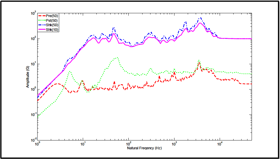
Figure description:
Vibration and Shock Response Curves Amplitude (G vs Natural Frequency (Hz
Shock Response Spectra Comparison
Legend
- Pre(50 — color: red; symbol: Dashed line
- Pst(50 — color: green; symbol: Dotted line
- Shk(50 — color: blue; symbol: Dash-dotted line
- Shk(10 — color: magenta; symbol: Solid line
| Natural Frequency (Hz) | Pre(50) | Pst(50) | Shk(50) | Shk(10) |
|---|---|---|---|---|
| 1 | 0.35 | 0.08 | 0.5 | 0.45 |
| 2 | 1.2 | 0.3 | 2.5 | 2.5 |
| 3 | 1.6 | 0.6 | 5.0 | 5.0 |
| 5 | 0.8 | 5.0 | 15.0 | 12.0 |
| 7 | 0.8 | 2.0 | 20.0 | 18.0 |
| 10 | 2.1 | 1.2 | 55.0 | 45.0 |
| 15 | 0.9 | 1.1 | 110.0 | 90.0 |
| 20 | 1.1 | 1.8 | 130.0 | 110.0 |
| 25 | 1.0 | 3.5 | 150.0 | 110.0 |
| 35 | 1.1 | 8.0 | 120.0 | 100.0 |
| 50 | 2.0 | 16.0 | 260.0 | 160.0 |
| 75 | 1.0 | 6.0 | 100.0 | 70.0 |
| 100 | 1.7 | 4.0 | 75.0 | 55.0 |
| 150 | 1.2 | 4.0 | 60.0 | 48.0 |
| 200 | 1.1 | 3.5 | 80.0 | 65.0 |
| 300 | 2.0 | 6.8 | 170.0 | 120.0 |
| 500 | 3.2 | 3.5 | 100.0 | 75.0 |
| 750 | 2.1 | 5.0 | 130.0 | 85.0 |
| 1000 | 4.8 | 6.5 | 140.0 | 100.0 |
| 1800 | 3.5 | 4.5 | 450.0 | 250.0 |
| 3500 | 12.0 | 15.0 | 650.0 | 400.0 |
| 5000 | 4.5 | 5.0 | 280.0 | 220.0 |
| 7500 | 2.5 | 6.5 | 150.0 | 120.0 |
| 10000 | 2.5 | 4.8 | 110.0 | 105.0 |
| 20000 | 2.5 | 4.5 | 100.0 | 100.0 |
| 50000 | 1.6 | 3.8 | 100.0 | 100.0 |
Notes: The chart is a log-log plot showing Amplitude (G versus Natural Frequency (Hz. The x-axis ranges from 1 to 50,000 Hz, and the y-axis ranges from 0.01 to 1,000 G.))
Figure 516.8A-7. Maximax acceleration SRS estimates for shock and noise floor segments.
As a time history validity check, Figure 516.8A-5 and Figure 516.8A-6 provides the positive and negative SRS estimates. It is noted that in these two figures neither the positive nor negative SRS value dominates the other; that would imply the time history information is valid.
1.5 Frequency Domain Identification Energy Spectral Density (ESD)
The ESD estimate is a properly scaled squared magnitude of the Fourier Transform of the total shock. Its counterpart, the Fourier Spectra (FS) is, in effect, the square root of the ESD, and may be useful for display but will not be discussed here. The importance of the ESD estimate is its properties relative to input/output system computations. That is for two acceleration measurements related as input and output, either (1) an estimate of the transfer function (magnitude/phase) between the input and output is possible, or (2) a transmissibility estimate (magnitude alone) can be determined by ratioing the output ESD over the input ESD. Further details and illustration of ESD estimates are provided in Annex B.
1.6 Single Event / Multiple Channel Measurement Processing Guidelines
When multiple measurements are made for a single configuration, generally pre-processing should proceed as if multiple channel analysis is to be performed. In particular, the pre-shock noise floor, the shock event, and the post- shock noise floor should be of the same duration, and this duration for the shock event should be determined based upon the "longest" duration measurement. Since SRS and ESD processing are generally insensitive to differences in the duration of significant energy content, such selection will allow multi-channel processing. It is imperative that for cross-energy spectral density estimates and energy transfer function estimates, the pre-processing, e.g., event selection durations, filtering, etc., on all measurement channels be the same. Pre-processing across multiple measurement channels involving integration of acceleration to determine velocity needs to correspond to the physics of the configuration. For high signal-to-noise ratios, useful information can be obtained from cross-spectral and transfer function estimates even though random error is high.
1.7 Measurement Probabilistic / Statistical Summary
Recommend that, whenever possible, two or more equivalently processed response measurements or test estimates be combined in some statistical manner for summary. This summary then can be used for test specification purposes to provide a level of confidence that the important information in the measurement or test has been captured. Paragraph 7.1, reference b, discusses some options in statistically summarizing processed results from a series of measurements
MIL-STD-810H
METHOD
1.8 Other Processing
Other descriptive processes that tend to decompose the shock into component parts, e.g., product model, time domain moments (TDM), wavelets, SRS modal and power energy methods (PEM), etc., may be useful, but details of such descriptive processes are beyond the scope of this document, and generally fall in the area of analytical modeling. TDM and PEM show promise of being able to characterize and compare individual shocks among sets of similar shock time traces and perhaps provide insight into cause of materiel failure from shock. TDM (paragraph 7.1, reference k) assessment provides for characterization of the “form” of measured response with respect to both time and frequency. PEM (paragraph 7.1, reference l) attempts to estimate the energy absorbed within a simple modal structure of the materiel when the materiel’s base attachment is the source of the shock input (or power input) to the materiel. PEM seems most useful for power comparison among similar measurements for shock, and has units (force*velocity) that relate to damage potential when applied to base motion relative to mass motion.