527.2-44 test process

527.2-4.1 Development of Mission or Lifetime Scenario

The duration of the vibration environments can be derived from the item’s Life Cycle Environment Profile (LCEP). The life cycle will include many different types of induced mechanical environments which may occur while the materiel is being handled, transported, deployed and operated. Although all the induced mechanical environments are not critical in terms of generating potential damaging response amplitudes, they contribute in varying degrees to the materiel’s fatigue damage. All expected exposure conditions should be tabulated, along with corresponding durations, to form the items lifetime “scenario”. The scenario is a key parameter in the development of any vibration schedule.

MIL-STD-810H

METHOD 527.2

design of the test set up, fixtures, transducer mountings, and wiring, along with good quality control will be necessary to meet the tolerances of paragraph 4.2.2 below.

527.2-4.2 Limitations

The mechanical degrees of freedom (DOFs) for which a VSD effort is capable of addressing, is a function of the number and placement of the transducers employed in the field data acquisition phase. Similarly, the maximum number of mechanical DOFs possible to reproduce in the laboratory environment is a function of the number and placement of actuators and coupling hardware. This Annex will consider the general case for VSD development in which the reference SDM will be defined in terms of the six classical (3-translational and 3-rotational) rigid body mechanical DOFs. In the event less than six mechanical DOFs are being considered, the generalized theory is easily configured to address the motion of interest.

MIL-STD-810H METHOD

4.2.1 Calibration

Ensure the excitation apparatus, all transducers, signal conditioning equipment, independent measurement systems, and the vibration control system are calibrated for conformance with the specified test requirement. Careful design of the test set up, fixtures, transducer mountings and wiring, along with good quality control will be necessary to meet the tolerances of paragraph 4.2.2 below.

4.2.2 Tolerances

The question of reasonable tolerances in a MET is not simple for either MET procedure. Guidelines for establishing test tolerances for a Procedure I MET are discussed in Annex C, and tolerances for a Procedure II MET are discussed in Annex D. Due to the unique factors associated with a MET, test metrics will often need to be addressed on a test by test basis. It is critical that the test objectives be clearly understood prior to establishing test tolerances, and that the metrics are carefully documented prior to conduct of the test.

527.2-4.3 Field Data Acquisition

When in-service measurement data have been obtained, it is assumed that the data is processed in accordance with good data analysis procedures, as in Multi-Shaker Test and Control IEST-RP-DTE022.18 and Welch's method. In particular, an adequate number of statistical degrees of freedom (DOFs) have been obtained to provide information with acceptable statistical error. Consideration must be given to not only statistical error in auto-spectral density estimates, but also in cross-spectral density estimates (including transfer and coherence function estimates).

4.3.1 Interruption Due To Laboratory Equipment Malfunction

• a. General. See Part One, paragraph 5.11, of this Standard.
• b. Specific to this Method. When interruptions are due to failure of the laboratory equipment, analyze the failure to determine root cause. It is also strongly advised that both control and response data be evaluated to ensure that no undesired transients were imparted to the test item during the test equipment failure. If the test item was not subjected to an over-test condition as a result of the equipment failure, repair the test equipment or move to alternate test equipment and resume testing from the point of interruption. If the test item was subjected to an over-test condition as a result of the equipment failure, immediately notify the test engineer or program engineer responsible for the test item. Conduct a risk assessment based on factors such as level and duration of the over-test event, spectral content of the event, cost and availability of test resources, and analysis of test specific issues to establish the path forward. See Method 514.8, Annex A, paragraph 2.1 for descriptions of common test types, and a general discussion of test objectives.

527.2-4.3.1 Instrumentation

For the purpose of this Annex, all instrumentation related discussions will be limited to linear accelerometers and engineering units of g's, as was the case in the general control discussion provided in paragraph 3.1.1. Linear accelerometers have several advantages including familiarity to most users, low cost, wide bandwidth, small size and weight, and readily available low cost highly reliable signal conditioning options.

4.3.2 Interruption Due To Test Item Operation Failure

Failure of the test item(s) to function as required during operational checks presents a situation with several possible options. Failure of subsystems often has varying degrees of importance in evaluation of the test item. Selection of options a through c below will be test specific.

• a. The preferable option is to replace the test item with a “new” item and restart the entire test.
• b. An alternative is to replace/repair the failed or non-functioning component or assembly with one that functions as intended, and restart the entire test. Conduct a risk analysis prior to continuing since this option places an over-test condition on the entire test item except for the replaced component. If the non-functioning component or subsystem is a line replaceable unit (LRU) whose life-cycle is less than that of the system test being conducted, proceed as would be done in the field by substituting the LRU, and continue from the point of interruption.
• c. For many system level tests involving either very expensive or unique test items, it may not be possible to acquire additional hardware for re-test based on a single subsystem failure. For such cases, a risk assessment should be performed by the organization responsible for the system under test to determine if replacement of the failed subsystem and resumption of the test is an acceptable option. If such approval is provided, the failed component should be re-tested at the subcomponent level.

MIL-STD-810H

METHOD 527.2

NOTE: When evaluating failure interruptions, consider prior testing on the same test item and any consequences of such.

4.3.3 Interruption Due To A Scheduled Event

There are often situations in which scheduled test interruptions will take place. For example, in a tactical transportation scenario, the payload may be re-secured to the transport vehicle periodically (i.e., tie-down straps may be re-secured at the beginning of each day). Endurance testing often represents a lifetime of exposure; therefore it is not realistic to expect the payload to go through the entire test sequence without re-securing the tie-downs as is done in a tactical deployment. Many other such interruptions, to include scheduled maintenance events, are often required over the life-cycle of materiel. Given the cumulative nature of fatigue imparted by dynamic testing, it is acceptable to have test interruptions that are correlated to realistic life-cycle events. All scheduled interruptions should be documented in the test plan and test report.

4.3.4 Interruption Due To Exceeding Test Tolerances

Exceeding the test tolerances defined in paragraph 4.2.2, or a noticeable change in dynamic response may result in a manual operator initiated test interruption or an automatic interruption when the tolerances are integrated into the control strategy. In such cases, check the test item, fixturing, and instrumentation to isolate the cause.

• a. If the interruption resulted from a fixturing or instrumentation issue, correct the problem and resume the test.
• b. If the interruption resulted from a structural or mechanical degradation of the test item, the problem will generally result in a test failure, and a requirement to re-test unless the problem is allowed to be corrected during testing. If the test item does not operate satisfactorily, follow the guidance in paragraph 4.3.2 for test item failure.

527.2-4.4 Use of Rigid Body Modes

• a. In single axis testing, the control input is often defined with a single accelerometer. This is satisfactory if the shaker and test fixtures are rigid within the frequency band of interest. If the shaker and test fixtures are not rigid, the technique of using a single accelerometer for control can sometimes lead to serious difficulty. To overcome these problems, methods using the average of several accelerometers and/or force limiting have come into common practice. In MEMA testing, the problem can be more serious as non-rigid body response is more common. When considering the special case of multiple shakers exciting a test item with multiple rigid body degrees of freedom, the use of the input transformation to define the response in terms of rigid body modes has several advantages. It is somewhat analogous to a generalization of the common practice for single axis testing. If there are more control channels than rigid body degrees of freedom, and an input transformation matrix is defined to transform the control accelerometers into rigid body modes, one essentially defines the motion of each rigid body mode as a weighted average of the accelerometers active for the mode. In many cases, given the control authority of the shakers, this is about the best viable solution. It is analogous to averaging accelerometers for a single axis test, which is common practice. The elastic modes are not controlled, since often the control authority over these modes does not exist. The system is driven with an equivalent rigid body motion in each of the rigid body modes. It is necessary to make sure that for any mode the transformation of the control accelerometers {a} does not result in zero for any of the rigid body modes. If higher flexural modes are present they will not be controlled. In theory the flexural modes can be limited by adding control variables, but this requires knowledge of the modes in the test setup. This information can only be determined with materiel in the test configuration. For this reason, it is sometimes desirable to allow modification of the test requirements after this information is made available. Exactly how this will be accomplished in specification writing will have to be determined at a later date.
• b. An advantage of using rigid body modes in the specification is that the field measurements used to define the environment can be made with the transducers in locations different from the locations of the transducers used in the laboratory test. The field measurements are reduced to equivalent rigid body modes using an acceleration transformation matrix (refer to paragraph 4.4.1), and the modes are controlled on the test using another transformation matrix for the laboratory test configuration. The two transformation matrices do not have to be the same. Use of alternate control points, while maintaining a full rank transformation matrix, provides a way of making the laboratory test “equivalent” in the sense of the rigid body modes.
• c. A practical difficulty arises when more modes are attempted to be controlled. The general case of six (6) rigid body modes requires the specification of a 6 x 6 SDM (6 ASD's and 15 CSD's). Physical understanding of the SDM matrix associated with rigid-body motion by itself is difficult without the additional complications of elastic DOFs. Furthermore, it is difficult to assure that the specification results in a positive definite SDM, which is a physical requirement. (Additional discussion on positive definite matrices is the subject of paragraph 4.5.2.)

4.4.1 Instrumentation

Various sensor types can be used in a MET setup and used to establish the need for a MET. In general, and used in examples throughout this document, acceleration will be the quantity measured to establish the specification for the procedure. Processed sensor measurement information from the lab environment should correspond to processed measurement information made in the field. This is ideally accomplished by mounting the test item accelerometer in the same location as that on the field measurement materiel from which the measured information was extracted. In the MDOF case, instrumentation location and polarity become critical test parameters (refer to Annex A). To maintain proper phase relationships between channels, a synchronous sample and hold analog to digital converter (A/D) is recommended. When possible, recommend laboratory and field data acquisition and instrumentation be the same. Otherwise, it may be necessary to precondition reference data prior to conduct of a laboratory test.

Calibrate all measurement instrumentation to traceable national calibration standards (see Part One, paragraph 5.3.2). The measurement device and its mounting will be compatible with the requirements and guidelines provided in paragraph 6.1, reference e.

• a. Accelerometer. In the selection of any transducer, one should be familiar with all parameters provided on the associated specification sheet. Key performance parameters for an accelerometer follow:
• (1) Frequency Response: A flat frequency response within ± 5 percent across the frequency range of interest is required.
• (2) Transverse sensitivity should be less than or equal to 5 percent.
• (3) Nearly all transducers are affected by high and low temperatures. Understand and compensate for temperature sensitivity deviation as required. Temperature sensitivity deviations at the test temperature of interest should be no more than ± 5% relative to the temperature at which the transducer sensitivity was established.
• (4) Base Strain sensitivity should be evaluated in the selection of any accelerometer. Establishing limitations on base strain sensitivity is often case specific based upon the ratio of base strain to anticipated translational acceleration.

MIL-STD-810H

METHOD 527.2

• (5) High sensitivity accelerometers are recommended when linear accelerometers are employed to make rotational motion estimates.
• b. Other measurement devices. Any other measurement devices used to collect data must be demonstrated to be consistent with the requirements of the test.

527.2-4.4.1 Acceleration (Input) Transformation

The acceleration to control space transformation matrix, T , commonly referred to as the “input transformation a matrix” from the control system perspective, is defined in the article “Applying Coordinate Transformations to Multi- DOF Shaker Control”9 and generalized in the article “Benefits and Challenges of Over-Actuated Excitation Systems”10. The acceleration transformation matrix transforms a set of accelerometer measurements into a set of

MIL-STD-810H

METHOD

4.4.1.1 Acceleration (Input) Transformation Derivation

One goal of this Annex is to define a standard nomenclature. The following summary has been restructured to the nomenclature defined by this Annex. Referring to the input transformation derivation10, a generic acceleration measurement at the k th position in orientation j is structured as Equation 4.1:

આ[ય [૯][] (4.1)

where $a_{0}$ is the linear acceleration at some reference point designated the "origin", $\alpha$ is the angular acceleration of the body (assuming it is rigid), $k \in\left(1,2, \ldots, N_{a}\right), i \in\left(1,2, \ldots, n^{*}\right), j \in(x, y, z)$, and $\mathbf{e}_{x}^{T}=[100], \mathbf{e}_{y}^{T}=[010]$, and $\mathbf{e}_{z}^{T}=[001]$ are row selection vectors (as shown assuming accelerometer orientation is aligned per a traditional right hand Cartesian system). Parameter $N_{a}$ represents the number of accelerometer measurements (as previously defined) and $n^{*} \leq N_{a}$ the number of measurement locations; e.g., utilization of multi-axis accelerometers results in $n^{*}<N_{a}$. Vector $r_{i}$ is the position vector relating the position of measurement location $i$ to a user defined origin. $\left[\begin{array}{c}^{P} \\ \boldsymbol{r}_{i}^{P}\end{array}\right]^{x}$ is the skew symmetric operator equivalent of the cross product, making the matrix based computations in Equation 4.1 possible. The matrix equivalent of a vector (i.e., a coordinatized vector quantity) is denoted as $\left(\begin{array}{c}() \\ ()\end{array}\right)_{\left(\right)}$ where the right superscript and subscript identify the body and point of interest respectively, and the left superscript denotes the coordinate frame in which the vector quantity was coordinatized; e.g., ${ }^{P} \boldsymbol{r}_{i}^{P}$ in Equation 4.1 denotes the i th point on body P (the platform) coordinatized in frame $\mathcal{F}_{p}$ - the platform's coordinate frame.

4.4.1.2 Equation 4.1

Equation 4.1 represents one equation in six unknowns, the three components of the linear acceleration of the reference point and the three components of the rigid body angular acceleration. In order to determine these quantities, at least six measurements are needed. These requirements are not as stringent as that reported in the article “On the Use of Linear Accelerometers in Six-DOF Laboratory Motion Replication”11 because of the assumptions above (i.e., small angular velocities and rigid body).

MIL-STD-810H

METHOD 527.2 ANNEX E

Let's consider the most general case of $N_{a}$ measurements from $n^{*}$ locations. In this case, Equation 4.1 becomes:

a [r] P a2 [] [ak,] = EXT... ‚ i ɛ (1, 2, ..., nº), j ɛ(x, y, z) ... P an (6x1) [[]] (nx1) (nx6)

which using the nomenclature defined in this Annex is of the form:

(4.2)

where {C}) Motion is a 6 x 1 matrix of unknown linear and angular accelerations and {a} Meas is an nxl matrix of acceleration measurements. Observe that [1] is entirely defined by knowledge of (i) placement, (ii) orientation, ¿] and (iii) utilized signals of the accelerometers.

Observe that if Tis of full column rank, then [TT]' exists enabling {C} Motion to be solved as follows:

$\begin{aligned} \left\{\mathbf{a}\right\}_{\text {Meas }} & =\overline{\mathbf{T}}_{\mathrm{a}}\left\{\mathbf{c}\right\}_{\text {Motion }} \\ \overline{\mathbf{T}}_{\mathrm{a}}^{\mathrm{T}}\left\{\mathbf{a}\right\}_{\text {Meas }} & =\overline{\mathbf{T}}_{\mathrm{a}}^{\mathrm{T}} \overline{\mathbf{T}}_{\mathrm{a}}\left\{\mathbf{c}\right\}_{\text {Motion }} \\ \left[\overline{\mathbf{T}}_{\mathrm{a}}^{\mathrm{T}} \overline{\mathbf{T}}_{\mathrm{a}}\right]^{-1} \overline{\mathbf{T}}_{\mathrm{a}}^{\mathrm{T}}\left\{\mathbf{a}\right\}_{\text {Meas }} & =\left[\overline{\mathbf{T}}_{\mathrm{a}}^{\mathrm{T}} \overline{\mathbf{T}}_{\mathrm{a}}\right]^{-1} \overline{\mathbf{T}}_{\mathrm{a}}^{\mathrm{T}} \overline{\mathbf{T}}_{\mathrm{a}}\left\{\mathbf{c}\right\}_{\text {Motion }} \\ \left[\overline{\mathbf{T}}_{\mathrm{a}}^{\mathrm{T}} \overline{\mathbf{T}}_{\mathrm{a}}\right]^{-1} \overline{\mathbf{T}}_{\mathrm{a}}^{\mathrm{T}}\left\{\mathbf{a}\right\}_{\text {Meas }} & =\left\{\mathbf{c}\right\}_{\text {Motion }}\end{aligned}$

Defining $\mathbf{T}_{\mathrm{a}} \equiv\left[\overline{\mathbf{T}_{\mathrm{a}}}^{\mathrm{T}} \overline{\mathbf{T}}_{\mathrm{a}}\right]^{-1} \overline{\mathbf{T}}_{\mathrm{a}}^{\mathrm{T}}$, Equation 4.2 can be rewritten as:

{C}Motion = [T]{a} Meas (4.3)

Where $\left[\mathbf{T}_{\mathrm{a}}\right]$ is a $6 \mathrm{X} n$ matrix referred to in the literature as the "Acceleration Transform Matrix" or "Input Transform

Matrix". Observe that the critical requirement that [TT] exists in order to derive the input transformation matrix

[

]

$\left[\mathbf{T}_{\mathrm{a}}\right]$, is solely a function of placement and orientation of measurement transducers.

4.4.2 Platform Integration

• a. Test Fixture Design. Observe standard shock and vibration fixture design practices with regard to frequency response and the ability to withstand the reaction forces with consideration of potentially high loads generated during MEMA tests as a result of the accelerations applied simultaneously in multiple degrees of freedom.
• b. Test Configuration. Both MESA and MEMA tests require that the test configuration be restrained in all degrees of freedom that are not controlled by the exciter, and released in all degrees of freedom that are. A kinematic assessment of the setup is recommended to assist in the selection of the proper couplings, bearings, etc., to ensure that improper loads are not transferred to the test item through the controlled application of the test, as well as the potentially uncontrolled motion of the exciters.

527.2-4.4.2 Drive (Output) Transformation

• a. Although details of the Drive Transformation are not required to develop a MDOF VSD reference, a short summary of the concept is provided for general knowledge. Referring to the schematic in Figure 2, transformation matrix Ts transforms the N drive variables into Ns shaker drive signals. Reference 10 d provides a formal derivation of the transformation matrix, Ts. Note that while the “acceleration transformation” was computed based on knowledge of position and polarity of the control accelerometers, the transformation matrix, Ts is dependent upon the position and line of action (LOA) of the individual actuators. In this Annex and within reference 10 Ts is referred to as the “drive transformation” or “output transformation”. The following cases summarize the computation of Ts and the effect on the control process.

MIL-STD-810H METHOD

4.4.2.1 Drive (Output) Transformation Derivation

• a. As previously stated, one goal of this Annex is to recommend a standard nomenclature. The following summary from reference number 10 has been restructured to the nomenclature recommended by this Annex. Figure 3 illustrates the generalized multi-axis vibration system.

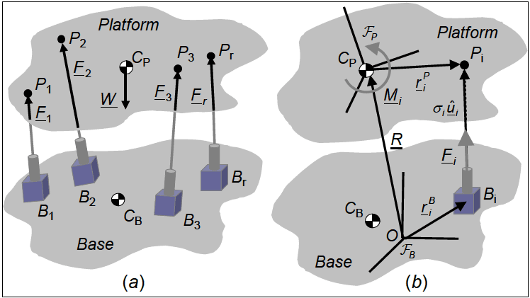
Figure description:

Key Entities and Details:

• System Components:

  • Base: Lower fixed structure with actuator mounting points $B_1, B_2, B_3, B_r$ and center of mass $C_B$.
  • Platform: Upper movable stage with attachment points $P_1, P_2, P_3, P_r$ and center of mass $C_P$.
  • Actuators: Links connecting the base to the platform, exerting forces $\underline{F}_i$.

• Kinematic and Dynamic Parameters:

  • Coordinate Frames: Base frame $\mathcal{F}_B$ at origin $O$; Platform frame $\mathcal{F}_P$ at $C_P$.
  • Position Vectors: $\underline{R}$ (Base origin to Platform center, $\underline{r}_i^B$ (Base origin to $B_i$, and $\underline{r}_i^P$ (Platform center to $P_i$.
  • Loading: Platform weight $\underline{W}$, actuator force $\underline{F}_i$, and resulting moment $\underline{M}_i$.
  • Actuator Geometry: Vector $\sigma_i \hat{u}_i$ defines the direction and extension from base point $B_i$ to platform point $P_i$.

Figure 3. Generalized multi-axis vibration system.

• b. Refer to reference number 10 for a detailed derivation of Equation 4.4. The following summary illustrates how the output transform, Ts is associated with the P-Matrix, (Plucker Matrix) discussed in the reference.

MIL-STD-810H

METHOD 527.2 ANNEX E

B P B B B m("-")-"FE

(4.4) P P P P P m₁ m 'L' à + ["] "L" (" ") - "ME | P =C

P F C 6xN Nx1 6x1

c. In Equation 4.4, $\left.\lbrack \mathbf{P}\right.\rbrack$ represents the Plucker Matrix which is derived from known geometric parameters associated with the individual actuators, $\left.\lbrack \mathbf{F}\right.\rbrack$ represents the drive and $\left.\lbrack \mathbf{C}\right.\rbrack$ represents the desired motion. The variables $^B\underline{\mathbf{\hat{u}}}_i$ represent the LOA vectors for each of the actuators and $^P\underline{\mathbf{m}}_i^P$ is the moment arm associated with force $f_i$. Observe that the maximum dimension for the $\left.\lbrack \mathbf{C}\right.\rbrack$ matrix will be six, if all six traditional motion DOFs are being considered (i.e. $N_d=6$ ). As stated in paragraph 4.4.2, Case 1 scenarios will simply have an identity matrix as the output transformation matrix and Case 3 scenarios (under-actuated) will not have a unique solution. Case 2 scenarios (over-actuated) may be addressed in terms of output transformations. The objective is to determine $\left.\lbrack \mathbf{F}\right.\rbrack$ in Equation 4.4, yielding the $N_s$ drive signals as follows:

T T (1) Define F P D and substitute into P F = C yielding P P D = C N₁x1 N₁x6 6x1 6xN, N₁x1 6.x1 6xN, N,x6 6x1 6x1

(2) $\underset{6 \times N_{s}}{\mathbf{P}} \underset{N_{s} \times 6}{\mathbf{P}^{T}}$ will be of full rank (i.e. invertible) if $\underset{6 \times 6}{[\mathbf{P}]}$ is of full rank.

(a) If [P] is of full rank: D = P P RP/ T T C 6x1 6xN, N₁x6 6x1

• (b) If [ ] P is not full rank, actuator placement is not sufficient to obtain the mechanical DOF’s desired.

(3) Substituting results from (2) yields $\mathbf{F} \equiv \underset{N_{s} \mathrm{x} 1}{\mathbf{P}^{T}} \underset{N_{s} \mathrm{x} 6}{\mathbf{D}}=\underset{N_{s} \mathrm{x} 6}{\mathbf{P}^{T}}\left[\begin{array}{cc}\underset{6 \mathrm{x} N_{s}}{\mathbf{P}} & \underset{N_{s} \mathrm{x} 6}{\mathbf{P}^{T}}\end{array}\right] \underset{6 \mathrm{x} 1}{\mathbf{C}}$

(4) $\underset{N_{s} \mathrm{x} 6}{\mathbf{T}_{s}} \equiv \underset{N_{s} \mathrm{x} 6}{\mathbf{P}^{T}}\left[\begin{array}{ll}\mathbf{P} & \mathbf{P} \\ 6 \mathrm{x} N_{s} & N_{s} \mathrm{x} 6\end{array}\right]$

• d. The discussions within this paragraph and previous derivation assumed Nd = 6. In the event Nd <6, Nd would represent the actual number of mechanical DOFs. In terms of the nomenclature of Figure 2, and assuming matched actuators are employed, voltage drives to the shakers for the over-actuated scenario would be defined as Equation 4.5:

4.5 Data Analysis.

• a. Ensure transducer placements have been addressed, to guarantee the desired motion DOFs may be resolved (refer to paragraph 4.4.1.2), and that common data validity checks are performed. Then, it is recommended that appropriate combinations of the linear acceleration measurements be transformed into the desired traditional motion DOFs through implementation of the acceleration transformation matrix. The transformed

MIL-STD-810H METHOD

4.4.3 Setup Analysis

In general, because of impedance mismatches and boundary condition effects, differences between the field and laboratory environments will exist. Such differences between the laboratory measured and test specified information may require further analysis with respect to the original field data and payload dynamics to determine if the differences are relevant to the test objectives.

• a. Rudimentary analysis to ensure the test tolerances are met is usually performed within the MET software and control strategy. Laboratory personnel should consult the vendor-supplied MET control system documentation, and clearly understand the determination of these test tolerances. In most cases this will require direct contact with the vendor of the MET system. At the time of this initial publication, common examples of analysis techniques that are performed during a MET include computation of EU-rms versus time, ASD, CSD, peak-detection, and histograms.
• b. More extensive data analysis can be performed to examine the significance of test tolerance deviations with off-line specialized software. Refer to Method 525.2, Annex B for Procedure I analysis methods, and paragraph 6.1, references d and e for a variety of detailed analysis techniques for random data applicable for Procedures I and II.

4.5.1 Preparation for Test

Carefully examine the reference time histories or specified auto- and cross-spectral information for validity. Ensure the test specification is band-limited according to the band limits of the shaker system. In particular, it may be necessary to remove any high amplitude low frequency components that will cause an over-travel condition for the shaker control system or result in velocity limit violation. In the event the reference data must be modified to address exciter system limitations, care must be exercised to ensure the intent of the test is not compromised; and the modifications must be documented and approved by the responsible test officer. Most MET systems do provide for such exciter system limit checks; however, the feasibility of exciter reproduction relative to cross-spectral information is generally not checked.

Characterize the materiel to be tested. For example:

• a. Dynamically flexible structure with a varying length/diameter ratio.
• b. Dynamically stiff structure with flexible appendages.
• C. Dynamically/geometrically asymmetric structure.
• d. Materiel in shipping or storage containers with pursuant materiel/container isolation.

If the test item is unique and must not be degraded before laboratory testing, test a dynamic simulation item that represents the dynamic properties of the materiel to be tested to ensure the MET can be properly compensated. Such a preliminary test will allow specification and refinement of the control strategy, including selection of control measurement points. It may also allow specification of the overall exciter configuration for optimizing the test strategy.

MIL-STD-810H

METHOD 527.2

527.2-4.5.1 Phase and Coherence Based Representations of CSD Terms

Although the off-diagonal terms of the SDM are computed in terms of a CSD, it is common among control system vendors to allow cross terms to be defined in terms of Phase and Coherence. This is a convenient option in that it is often easier to physically interpret SDM CSD terms in terms of Phase and Coherence. There is a direct relationship between the two techniques of defining the cross terms of the SDM that is dependent upon the definition of ordinary

coherence between two signals, $\gamma_{ij}^{2}=\frac{\left|G_{ij}\right|^{2}}{G_{ii}G_{jj}}$ . Normalizing the CSD terms of the SDM by $\sqrt{G_{ii}G_{jj}}$ yields a normalized spectral density matrix $\left(\mathrm{SDM}_{\mathrm{n}}\right)$ in which the ASD terms are not affected and the magnitude of the normalized CSD terms are defined as $\frac{G_{ij}}{\sqrt{G_{ii}G_{jj}}}$ , which is equivalent to the square root of the ordinary coherence

function, while not affecting the original phase relationship of the CSD terms. Similarly, the normalized spectral density matrix, $\operatorname{SDM}_{\mathrm{n}}$, may be transformed back to the original CSD form of the SDM.

4.5.1.1 Preliminary Steps

Before starting a test, review pretest information in the test plan to determine test details (procedure(s), test item configuration(s), levels, durations, vibration exciter control strategy, failure criteria, test item operational requirements, instrumentation requirements, facility capability, fixture(s), etc.).

• a. Select the appropriate MET configuration and associated fixturing.
• b. Select the appropriate data acquisition system (e.g., instrumentation, cables, signal conditioning, recording, and analysis equipment).
• c. Operate vibration equipment without the test item installed to confirm proper operation.
• d. Ensure the data acquisition system functions as required.

4.5.1.2 Pretest Standard Ambient Checkout

All items require a pretest standard ambient checkout to provide baseline data. Conduct the pretest checkout as follows:

• Step 1 Examine the test item for physical defects, etc., and document the results.
• Step 2 Prepare the test item for test, in its operating configuration if required, as specified in the test plan.
• Step 3 Examine the test item/fixture/excitation system combination for compliance with test item and test plan requirements.
• Step 4 If applicable, conduct an operational checkout in accordance with the test plan and document the results for comparison with data taken during or after the test. If the test item fails to operate as required, resolve the problems and repeat the operational checkout.

4.5.2 Procedure

The following steps provide the basis for collecting the necessary information concerning the platform and test item under MET testing.

• a. Procedure I – Time Domain Reference Criteria.

• Step 1 Select the test conditions to be addressed and mount the test item on the excitation platform. Select the control locations and associated analysis techniques that will be used as potential test metrics (refer to Method 525.2, Annex A, and Annexes A, B, and C of this Method). Placement and polarity of all sensors (i.e. accelerometers) must match that of the reference signals (refer to Annex A). Clearly identify each axis of excitation and provide alignment procedures to ensure all measurements are made precisely along each excitation axis. Use all inherent information concerning the dynamic/geometric configuration of the test item, including specification of the center-of-gravity of the test item in three orthogonal axes, modal characteristics of the test fixturing, and all pertinent mass moments of inertia.

• Step 2 If required; perform an operational check of the test item at defined environmental test conditions per the test plan. If the test item operates satisfactorily, proceed to Step 3. If not, resolve the problem(s) and repeat this step.

• Step 3 Subject the test item (or dynamic simulant) to a system identification process that determines the initial exciter drive voltage signals by compensation. For the MDOF case, the initial signals sent to the exciters for compensation must be statistically independent, and form vectors that are linearly independent with respect to the DOFs to be tested. If a dynamic simulant is used, replace the dynamic simulant with the test item subsequent to the system identification and compensation phase.

• Step 4 Subject the test item in its operational mode to the TWR compensated waveform. It is often desirable to make an initial run at less than full level to ensure proper dynamic response, and to validate proper functioning of the instrumentation.

• Step 5 Record necessary data, including the control sensor time traces that can be processed to demonstrate that satisfactory replication of the matrix of reference time trace signals has been obtained.

• Step 6 Continuously monitor vibration levels and, if applicable, test item performance throughout the exposure. If levels shift or a failure occurs, shut down the test in accordance with the test interruption procedure (paragraph 4.3.2). Determine the reason for the shift and proceed in accordance with the test interruption recovery procedure (paragraph 4.3.2).

Step 7 Repeat Steps 4, 5, and 6 as specified in the test plan.

Step 8 Remove the test item from the fixture and perform an operational check. Inspect the test item, mounting hardware, packaging, etc., for any signs of visual mechanical degradation that may have occurred during testing. See paragraph 5 for analysis of results.

b. Procedure II – Frequency Domain Reference Criteria

• Step 1 Select the test conditions to be addressed and mount the test item on the excitation platform. Select the control locations and associated analysis techniques that will be used as potential test metrics (refer to Annexes A, B, and D of this Method). Placement and polarity of all sensors (i.e. accelerometers) must match that of the reference signals (refer to Annex A). Clearly identify each axis of excitation and provide alignment procedures to ensure all measurements are made precisely along each excitation axis. Use all inherent information concerning the dynamic/geometric configuration of the test item, including specification of the center-of-gravity of the test item in three orthogonal axes, modal characteristics of the test fixturing, and all pertinent mass moments of inertia.
• Step 2 If required; perform an operational check on the test item at defined environmental test conditions per the test plan. If the test item operates satisfactorily, proceed to Step 3. If not, resolve the problem(s) and repeat this step.
• Step 3 Subject the test item (or dynamically accurate surrogate if available) to a system identification process. For the MDOF case, the initial signals sent to the exciters must be statistically independent and form vectors that are linearly independent with respect to the DOFs to be tested. If a dynamic simulant is used, replace the dynamic simulant with the test item subsequent to the system identification and compensation phase.
• Step 4 Subject the test item in its operational mode to the specification levels, monitoring both auto and cross-spectral density terms. It is almost always necessary to make an initial run at less than full level to ensure proper dynamic response, and to validate proper functioning of the instrumentation.
• Step 5 Record necessary data, including the control sensor auto and cross-spectral estimates that demonstrate satisfaction of the overall test objectives.
• Step 6 Continuously monitor vibration levels and, if applicable, test item performance throughout the exposure. If levels shift or a failure occurs, determine the reason for the shift, and follow the test interruption procedure (paragraph 4.3.2).

Step 7 Repeat Steps 4, 5, and 6 as specified in the test plan.

• Step 8 Remove the test item from the fixture and perform an operational check. Inspect the test item, mounting hardware, packaging, etc., for any signs of visual mechanical degradation that may have occurred during testing. See paragraph 5 for analysis of results.

527.2-4.5.2 Positive Definite SDM Considerations

• a. Any specified spectral density matrix must be positive semi-definite to be physically realizable. In practice it must be positive definite. The determinate of the matrix must be ≥0. All the eigenvalues of the SDM must be ≥0. This must be true at all frequencies. It must be possible to perform a Cholesky decomposition of the specified SDM. Another property of positive semi definite matrices is from Matrix Computations12:

$\leq \Phi_{i i} \Phi_{j j} \quad \text { or } \quad 0 \leq \gamma^{2}=\frac{\left|\Phi_{i j}\right|}{\Phi_{i i} \Phi_{j j}} \leq 1$

2

In the terms of random vibrations the ordinary coherence, $\gamma^{2}$ between signals must be less than or equal to one. In practical terms, if the coherence between any pair of signals is one, the SDM will be positive semi-definite and the control system will have problems. Note that in general, if D is Hermitian and positive semi-definite C will also be Hermitian and positive semi-definite.

• b. If all the eigenvalues are non-negative, the matrix is positive semi-definite. If any of the eigenvalues are zero, it implies that one or more of the rows of the spectral density matrix are a linear combination of other rows. In practice, one would typically expect to deal only with positive definite matrices. Observe that even a small amount of noise or nonlinearity will result in a positive definite matrix. If a matrix is positive definite, the matrix can always be factored using Cholesky decomposition,

$\Phi=\mathrm{LL}^{\prime}$

where $\mathbf{L}$ is a lower triangular matrix. Which without loss of generality can be rewritten as,

Φ = LIL'

where I is the identity matrix. In this application, I is not really the identity matrix. I is a spectral density matrix. At every frequency, I is a diagonal matrix of ones. The components in I are independent since all the off diagonal elements are zero. It is now clear why the cross spectral density matrix must be positive definite. If any of the elements in I are zero, it implies that there are less than N (the number of rows or columns in $\Phi$ ) independent sources in $\Phi$. Some of the rows and columns are linear combinations of other rows and columns. The identity matrix is positive definite, therefore $\Phi$ must be positive definite. Using the interpretation of Random Data Analysis and Measurement Procedures ${ }^{13}$, the diagonal elements of I can be

MIL-STD-810H

METHOD

4.5.3 Data Compression

• a. Use of time compression techniques such as Miner-Palmgren may be employed to modify the ASD terms. References numbers 1 and 3 provide discussions on time compression. In the simplest terms, the Miner- Palmgren Hypothesis (Miner’s rule) is a set of mathematical equations used to scale vibration spectra levels and their associated test times. It provides a convenient means to analyze fatigue damage resulting from cyclical stressing. The mathematical expression and variable descriptions for this technique are illustrated in Equation 4.6:

$\frac{t_{2}}{t_{1}}=\left[\frac{S_{1}}{S_{2}}\right]^{M}$

(4.6)

where:

1t = equivalent test time

• $t_{2}=$ in-service time for specified condition

MIL-STD-810H METHOD

4.5.4 Limiting Strategies

Traditional notching techniques may also be employed if impedance mismatches lead to unrealistically high test item response. Notching techniques may be employed across all actuators with equal weighting or by weighting notching at each actuator as a function of coherence between the actuators and the location of interest. In addition to traditional notching based on acceleration spectra, it is also possible to consider limiting based on other parameters (e.g. von Mises Stress or Force limiting). As with any notching scheme, it is critical that any resulting deviations to the test or test tolerances must be approved by the appropriate test authority and must be clearly documented in the test plan and final report.

4.5.5 Minimum Drive Considerations

A number of challenges have been identified in addressing the objective of establishing a reference SDM for multiple exciter test (MET) scenarios. One major area of concern is related to the fact that it is highly likely that there will be mechanical impedance differences between the field and laboratory conditions. Given these impendence mismatch issues, it is undesirable to force the test item into what could potentially be an unnatural state as fixtured in the laboratory. Optimally, achieving the specified autospectra without excessively taxing the excitation system is desired. Smallwood made a general approach to establishing minimum drive criteria in the article “MIMO Linear Systems Extreme Inputs/Outputs”14. Unfortunately, the technique does not always guarantee the resulting SDM to be positive semi-definite.

4.5.5.1 Independent Drives

• a. Although an active area of research, general techniques to address minimum drive criteria have not been formally established at the time of this publication. A proposed approach for trending drive voltages towards minimums while maintaining a positive- definite SDM, is discussed in the article “A Proposed Method to Generate a Spectral Density Matrix for a MIMO Vibration Test”15, and is summarized below:
• (1) Taking a clue from the modal test community, assume the drive signals to the excitation system will be uncorrelated. Typically for a vibration test, the drives are the voltage inputs to the shakers. For a simulation, the inputs into a model are often forces. It is always possible to excite the system with uncorrelated inputs. This is standard practice in the modal community, and is standard practice when performing the system identification for MIMO test systems. This leads to the logical question: Is it possible to generate a set of uncorrelated inputs that will produce a desired set of response autospectra (the diagonal of the output SDM)?
• (2) The general equation relating the control point accelerations to the drive voltages is given in Random Vibrations, Theory and Practice16:

$\mathbf{S}_{\mathrm{y}}=\mathrm{HS}_{\mathrm{x}} \mathrm{H}^{\prime}$

where H' is the conjugate transpose of H , and SX and SY are SDM’s. H is a matrix of frequency response functions relating the output to the input of the excitation system. In our case, ideally, SX will be a diagonal matrix. Let X be a column vector of the diagonal of SX or, X = diag( S X ) , and

MIL-STD-810H METHOD

MIL-STD-810H METHOD

MIL-STD-810H METHOD