9.1 VSD Considerations
The VSD process will depend on several factors, including the vibration environment, system goals, value of the hardware, system fragility, test schedule constraints, test lab capabilities, and other considerations. Independent of the methods utilized, the results must define the vibration in laboratory testable terms and include a definition of the vibration levels and test exposure times.
The objective in the VSD effort outlined in Annex F, Appendix D, as opposed to a simple statistical combination of spectra exercise, is development of both a spectral reference and associated test time. As stated above in Annex F, paragraph 1, time compression techniques based on fatigue equivalency are typically employed such that vibration testing can be performed in a timely and economic manner. However, regardless of the VSD technique employed, one would expect the spectral shape of the final product to be similar to that of the field data used as the basis for the development. As a sanity check, one may wish to compare the spectral shape resulting from a VSD development to a basic statistical summary of the uncompressed reference data. Annex F, Appendix B provides a basic discussion on the topic of statistical combination of data that often proves useful in reviewing VSD spectral results. Annex F, Appendix C provides a discussion of combination of data from a Fatigue Damage Spectrum (FDS) perspective.
MIL-STD-810H
METHOD 514.8, ANNEX F
9.2 Engineering Data Common Across VSD Methods
The Handbook for Dynamic Data Acquisition and Analysis (reference 1) provides a wealth of signal analysis techniques and overall data acquisition guidance and is recommended as a key reference in the VSD process. A few of the most common analysis definitions utilized in VSD efforts are provided in Annex F, Appendix B.
9.2.1 Miner-Palmgren Hypothesis
In the simplest terms, the Miner-Palmgren Hypothesis (Miner’s rule) is a set of mathematical equations used to scale vibration spectra levels and their associated test times. It provides a convenient means to analyze fatigue damage resulting from cyclical stressing. Miner’s rule, originally based on empirical data, establishes a relationship between the ratio of the number of cycles at a given stress level to the number of cycles at another stress level.
The major cause of items failing to perform their intended function is material fatigue and wear accumulated over a time period as a result of vibration-induced stress. It is preferable for materiel to be tested in real-time so the effects of in-service conditions are simulated most effectively. However, in most instances real-time testing cannot be justified based on cost and/or schedule constraints and, therefore, it is customary to compress the service life environment into an equivalent laboratory test. For vibration environments that vary in severity during the materiel’s service life, the duration of the environment can often be reduced for testing by scaling the less severe segments of the vibration environment to the maximum levels of the environment by use of an acceptable algorithm.
In many cases, scaling less severe segments to the maximum levels may still yield a test duration that is still too long to be practical. In such cases, the same algorithm may be used to further reduce test duration by further increasing the test amplitude. Provided that fatigue is a significant potential failure criterion for the materiel under test, this practice is acceptable within strict limits, notably that test amplitudes are not over exaggerated (or accelerated) simply to achieve short test durations. Such excessive amplitudes may lead to wholly unrepresentative failures, and cause suppliers to design materiel to withstand arbitrary tests rather than the in-service conditions. Conversely, overly extending test durations in order to excessively reduce the amplitude may result in the test article passing vibration testing in the laboratory but experience vibration related failures in the field.
While the use of Miner’s rule is based upon fatigue damage being the principal failure mechanism, it has been found historically that test durations calculated by this means tend to be somewhat conservative when considering other failure mechanisms such as fretting and other types of wear. However, when considering the wide range of dynamic forcing functions considered over the life cycle of most hardware, test durations calculated using Miner’s rule have proven to be generally acceptable regardless of the failure mechanism under consideration.
9.2.1.1 S/N Curve
Graphically, the relationship of stress to number of cycles can be depicted as shown in Figure 514.8F-2. Figure 514.8F-2 relates stress (S) to the number of cycles (N) and is an example of a plot commonly referred to as the S/N curve. The black curve of Figure 514.8F-2 is the theoretical relationship of stress and the number of cycles. The red curve is a linearized representation of the black curve. Note that the number of cycles increases as the stress level decreases. At point A on the curve the stress level is so high that fatigue failure will result from any number of cycles. At point B on the curve, commonly referred to as the endurance limit, the stress level is so low that an infinite number of cycles will induce no fatigue damage. Between points A and B is the region of interest for Miner’s rule calculations.
MIL-STD-810H METHOD 514.8, ANNEX F
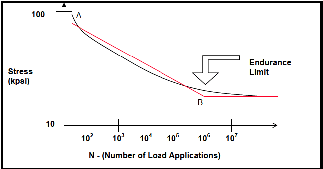
Figure description:
Fatigue Life S-N Curve with Endurance Limit
Stress vs. Number of Load Applications (S-N Curve
Legend
- Experimental Fatigue Curve — color: black; symbol: Solid line
- Idealized/Bilinear S-N Curve — color: red; symbol: Solid line
Annotations
- A (text_label - position: N ≈ 30, Stress ≈ 95)
- B (text_label - position: N = 10^6, Stress = 25)
- Endurance Limit (text_label - position: N > 10^6, Stress ≈ 25)
| N - (Number of Load Applications) | Stress - Black Line (kpsi) | Stress - Red Line (kpsi) |
|---|---|---|
| 3.00E+01 | 95.0 | 85.0 |
| 1.00E+02 | 70.0 | 78.0 |
| 1.00E+03 | 53.0 | 60.0 |
| 1.00E+04 | 40.0 | 45.0 |
| 1.00E+05 | 31.0 | 34.0 |
| 1.00E+06 | 27.0 | 25.0 |
| 1.00E+07 | 25.5 | 25.0 |
| 1.00E+08 | 25.0 | 25.0 |
Notes: The graph uses a logarithmic scale for both the Stress (y-axis and the Number of Load Applications (x-axis. Point B marks the knee of the bilinear approximation, commonly associated with the endurance limit for materials like steel.))
Figure 514.8F-2. S/N curve.
9.2.1.2 Miner-Palmgren Equations
The most commonly used method for calculating a reduction in test duration is the Miner-Palmgren hypothesis that uses a fatigue-based power law relationship to relate exposure time and amplitude. The mathematical expression and variable descriptions for this technique are illustrated below in Equations (9.1) and (9.5).
た (9.1) t₁
where:
- equivalent test time
t₁ = in-service time for specified condition
S₁ = severity (rms) at test condition
at in-service condition
[The ratio S₁/S2 is commonly known as the exaggeration factor.]
m = a value based on (but not equal to) the slope of the S/N curve for the appropriate material where S represents the stress amplitude and N represents the mean number of constant amplitude load applications expected to cause failure.
In practice, vibration test amplitudes and durations need to be rescaled without knowledge of the original in-service condition (S2). Equation 9.2 is the generalized relationship for rescaling sine tone test amplitudes based on the original time compression and new time compression.
1 4t2 new ms Sinew = S₁ (9.2) t2t1new
where:
- original test time
t₂ original in-service time used to develop test
S₁ original test levels
(Historical materiel exponent for sinusoidal vibration, see Annex A, paragraph 2.2. The same material exponent value should be used when rescaling as used during the initial compression.)
tinew new test time
new in-service time on LCEP
rescaled test levels based on LCEP
MIL-STD-810H
Fatigue damage can be calculated using either a stress life or strain life process. Although most engineering structures are designed such that the nominal loads remain elastic, it is important to acknowledge that stress concentrations often cause plastic strains to develop in the vicinity of notches. Figure 514.8F-3 illustrates the total strain as a sum of plastic and elastic components of strain (reference o).
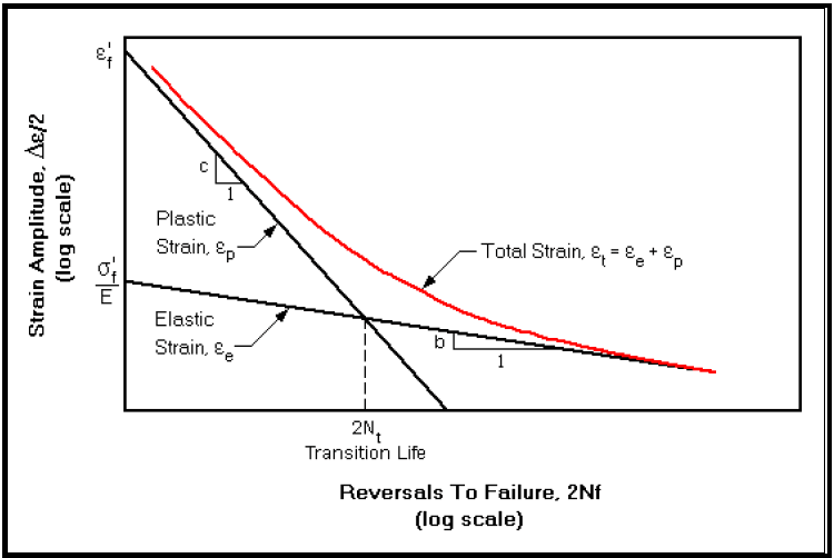
Figure description:
Fatigue Life Components Strain Amplitude vs. Reversals To Failure (log-log scale
Strain-Life Fatigue Diagram
Legend
- Total Strain, — color: red; symbol: Solid line
- Plastic Strain, — color: black; symbol: Solid line
- Elastic Strain, — color: black; symbol: Solid line
Annotations
- Plastic Strain slope: c (slope_indicator - position: on curve )
- Elastic Strain slope: b (slope_indicator - position: on curve )
- Transition Life, (vertical_line - position: x = )
- (text_label - position: y-intercept for plastic strain at )
- (text_label - position: y-intercept for elastic strain at )
| Reversals To Failure, (log scale) | Plastic Strain, | Elastic Strain, | Total Strain, |
|---|---|---|---|
| 1 | |||
| (Transition Life) | Intersection Value | Intersection Value | (Intersection Value) |
| High Cycles () | Low | High | |
| Low Cycles () | High | Low |
Notes: The graph depicts the standard strain-life fatigue model, showing how total strain is partitioned into elastic and plastic components on a log-log scale. The plastic strain follows the Manson-Coffin relation, while the elastic strain follows Basquin's equation.
Figure 514.8F-3. Typical strain life curve.
For the strain life technique (assuming zero static load), the number of cycles to failure, , is computed from: (9.3)
where: = test or environment strain amplitude = fatigue strength coefficient (material property) = modulus of elasticity (material property) = number of cycles to failure = fatigue strength exponent (material property) = fatigue ductility coefficient (material property) = fatigue ductility exponent (material property)
In equation 9.3, , represents elastic components on the strain-life, while , represents the plastic components. In the event a static load is present, Equation 9.3 may need to be compensated using techniques such as the Smith-Topper-Watson mean stress correction (reference n).
The transition life, , represents the life at which the elastic and plastic strain ranges are equivalent. The transition point of the two components of strain can be computed as:
2N₁ = [ɛ'‚E / σ', ] ½ (b−c) 1/(b-c)
(9.4)
As shown in Figure 514.8F-3, the transition life provides a convenient delineation between low and high-cycle fatigue. Plastic strains have greater influence below the transition life and Elastic strains have a greater influence above the transition life. For long fatigue lives, the strain-life approach will essentially approach the stress-life approach.
The value of in Equation 9.1 is strongly influenced by the material S/N curve, but fatigue life is also influenced by the surface finish, the treatment, the effect of mean stress correction. Figure 514.8F-4 graphically depicts the effects of finishing options on SAE-8630 steel to illustrate influence of surface finish on parameter .
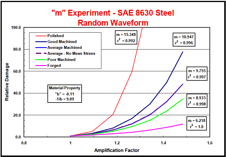
Figure description:
"m" Experiment - SAE 8630 Steel Random Waveform
"m" Experiment - SAE 8630 Steel Random Waveform
Legend
- Polished — color: red; symbol: Solid line
- Good Machined — color: dark blue; symbol: Solid line
- Average Machined — color: blue; symbol: Solid line
- Average - No Mean Stress — color: purple; symbol: Dashed line
- Poor Machined — color: green; symbol: Solid line
- Forged — color: magenta; symbol: Solid line
Annotations
- Material Property: "b" = -0.11, -1/b = 9.09 (text_label - position: x ≈ 1.05, y ≈ 35.0)
- m = 15.348, r² = 0.992 (text_label - position: x ≈ 1.25, y ≈ 90.0)
- m = 10.947, r² = 0.996 (text_label - position: x ≈ 1.5, y ≈ 90.0)
- m = 9.755, r² = 0.997 (text_label - position: x ≈ 1.5, y ≈ 65.0)
- m = 8.933, r² = 0.998 (text_label - position: x ≈ 1.5, y ≈ 40.0)
- m = 6.218, r² = 1.0 (text_label - position: x ≈ 1.5, y ≈ 15.0)
| Amplification Factor | Polished | Good Machined | Average Machined | Average - No Mean Stress | Poor Machined | Forged |
|---|---|---|---|---|---|---|
| 1.0 | 1.0 | 1.0 | 1.0 | 1.0 | 1.0 | 1.0 |
| 1.1 | 5.2 | 3.5 | 3.0 | 3.0 | 2.5 | 1.8 |
| 1.2 | 20.5 | 9.0 | 6.8 | 6.8 | 5.5 | 3.2 |
| 1.3 | 60.0 | 20.2 | 14.5 | 14.5 | 11.0 | 5.2 |
| 1.35 | 98.0 | 30.0 | 20.0 | 20.0 | 15.0 | 6.5 |
| 1.4 | null | 46.5 | 29.5 | 29.5 | 20.5 | 8.5 |
| 1.48 | null | 78.0 | 48.2 | 48.2 | 35.0 | 11.8 |
Notes: The chart shows Relative Damage vs. Amplification Factor for various surface finishes. Note that the 'Average Machined' and 'Average - No Mean Stress' series overlap significantly on the plot. The 'm' values represent the slope or exponent of the fatigue damage power law.
Figure 514.8F-4. Relative damage as a function of surface finish – SAE-8630 steel.
The combined contributions of elastic and plastic strain, and the waveshape of the strain time history, will also influence the value of m. Using SAE-8630 steel as an example, Figure 514.8F-5 graphically depicts the influence of the plastic component of strain on parameter m as strain levels approach the transition point.
MIL-STD-810H METHOD 514.8, ANNEX F
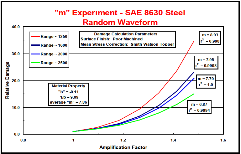
Figure description:
"m" Experiment - SAE 8630 Steel Random Waveform
"m" Experiment - SAE 8630 Steel Random Waveform
Legend
- Range ~ 1250 — color: red; symbol: Solid line
- Range ~ 1600 — color: dark blue; symbol: Thick solid line
- Range ~ 2000 — color: blue; symbol: Solid line
- Range ~ 2500 — color: green; symbol: Solid line
Annotations
- m = 8.93, r² = 0.998 (text_label - position: End of Range ~ 1250 curve)
- m = 7.95, r² = 0.9998 (text_label - position: End of Range ~ 1600 curve)
- m = 7.70, r² = 1.0 (text_label - position: End of Range ~ 2000 curve)
- m = 6.87, r² = 0.9994 (text_label - position: End of Range ~ 2500 curve)
- Material Property: "b" = -0.11, -1/b = 9.09, average "m" = 7.86 (text_label - position: x = 1.1, y = 14)
- Damage Calculation Parameters: Surface Finish: Poor Machined, Mean Stress Correction: Smith-Watson-Topper (text_label - position: x = 1.2, y = 35)
| Amplification Factor | Range ~ 1250 | Range ~ 1600 | Range ~ 2000 | Range ~ 2500 |
|---|---|---|---|---|
| 1.0 | 1.0 | 1.0 | 1.0 | 1.0 |
| 1.1 | 2.5 | 2.2 | 2.0 | 1.8 |
| 1.2 | 5.5 | 4.5 | 4.1 | 3.6 |
| 1.3 | 11.2 | 8.8 | 7.8 | 6.2 |
| 1.4 | 21.0 | 15.5 | 13.8 | 10.5 |
| 1.48 | 34.8 | 23.2 | 20.8 | 15.2 |
Notes: The data points are estimated from the visual plot. The x-axis represents the Amplification Factor and the y-axis represents Relative Damage.
Figure 514.8F-5. Relative damage as a function of strain range - SAE-8630 steel.
As a result of multiple factors such as finishing and actual strain levels, the value of m is generally some proportion of the slope of the S/N curve, known as the fatigue strength exponent and designated as b. Typical values of m are 80 percent of 1/b for random waveshapes, and 70 percent of 1/6 for sinusoidal waveshapes.
Historically, values of between 5 and 8 are commonly used when addressing random environments. A value in the range of 6 is commonly used for sinusoidal environments (references b, h and p).
The basis for the default recommendations in Table 514.8F-III may be traced to historical success of selections within the range suggested in Table 514.8F-III, combined with investigating the properties of a wide range of steel and aluminum alloys as discussed in reference n. Reference n summarizes a strain analysis that was conducted on an ensemble of commonly used steels and aluminum alloys in which strain levels approaching the transition life were considered. Strain levels in the analytical investigation of reference n were controlled such that the minimum number of cycles to failure was generally greater than 10,000 . Multiple finishing processes were considered as well. The default values in Table 514.8F-III have been separated into families of steel and aluminum alloys to add some fidelity in the selection of . Observe that historical values of 5-8 fall within the range of defined in Table 514.8F-III, providing an additional level of confidence between the historical values used for and the recent analytical study of reference n.
| Excitation Type | m - (Default Value) (Steels) | m - (Default Value) (Aluminum Alloys) |
|---|---|---|
| Sinusoidal | 5.75 | 8.5 |
| Random | 7 | 9 |
MIL-STD-810H
When addressing a LVTS for a simple test article whose design consists of a single material, one could simply look up the value of directly, and compute as a percentage (70-80 percent) of the inverse of as discussed above. The difficulty common to most LVTS development efforts of complex systems is that more than one material comprises the system design. In such cases, default values for parameter are recommended per Table 514.8F-III. If the exact composition of a complex structure is not known, it is recommended that the more conservative selections for based on steel are selected.
The cumulative damage assumption is based on the fatigue properties of metals. The Shock and Vibration Handbook, chapter 35 (reference d), recommends that Miner’s cumulative damage theory not be used for composite materials. However, a “wearout model,” defined as “the deterioration of a composite structure to the point where it can no longer fulfill its intended purpose,” is shown as a power law model in the form of Equation (9.1) with variable exponents dependent upon the type of composite system. It is recommended that test time compression for composite structures be treated on a case-by-case basis.
Since most vibration environments are expressed in terms of the auto spectral density function, Equation (9.1) can also be formulated as:
\right.} (9.5)
where:
The ratio of to becomes the exaggeration factor. For factors greater than 1 , the laboratory test time is reduced and conversely, for factors less than 1 , the test time is increased.
In practice, vibration test amplitudes and durations need to be rescaled without knowledge of the original in-service condition W(f)2. Equation 9.6 is the generalized relationship for rescaling the random broadband background based on the original time compression and the new time compression.
W(f)\new ₁ =W (ƒ)₁| t₁t 2 new (9.6) t2t\new
where: t₁original test time t2=original in-service time W(f)₁original test levels MR = 7.5 (Historical materiel exponent for random vibration, see Annex A, paragraph 2.2. The same material exponent value should be used when rescaling as used during the initial compression.) tinew new test time t2new new in-service time W(f)1new rescaled test levels based on LCEP
Selection of exponent m does not give complete freedom to the use of equations (9.1) and (9.5) in compressing test times! Caution must be exercised in using the exaggeration factor. It appears foolish to attempt to compress test time so that
increased amplitude will exceed the yield or ultimate strength of the material. Reference h, suggests limiting the exaggeration of test levels so as not to exceed the ratio of ultimate strength to endurance strength of the material being tested. In an attempt to determine a value for the maximum exaggeration factor, a search was conducted of the mechanical properties of 25 metals that have been used most often in a large variety of test items (reference i).
The ratios of ultimate stress (U) to the elastic limit (Y) and ultimate stress (U) to the endurance limit (EN) were calculated for each of the metals and averaged, producing values of U/Y = 1.37 and U/EN = 2.78. These ratios were then averaged, producing a value of 2.08 (see Table 514.8F-IV). The value of 2 is therefore suggested as the maximum limit for exaggeration factors.
| ELASTIC ENDURANCE | |||||
|---|---|---|---|---|---|
| LIMIT (Y) | LIMIT (EN) | ULTIMATE (U) | RATIO (U/Y) | RATIO (U/EN) | |
| Steel, 0.4% C, h. rolled | 53 | 38 | 84 | 1.59 | 2.21 |
| Steel, stainless (18-8) annealed | 36 | 40 | 85 | 2.36 | 2.13 |
| Steel, stainless (18-8) cold rolled | 165 | 90 | 190 | 1.15 | 2.11 |
| Alum, cast, 195T-6 | 24 | 7 | 36 | 1.33 | 5.14 |
| Alum, wrought, 2014-T4 | 41 | 18 | 62 | 1.51 | 3.44 |
| Alum, wrought, 2024-T4 | 48 | 18 | 68 | 1.42 | 3.78 |
| Alum, wrought, 6061-T6 | 40 | 13.5 | 45 | 1.13 | 3.33 |
| Magnesium, extrusion, AZ80X | 35 | 19 | 49 | 1.40 | 2.58 |
| Magnesium, sand cast, AZ63-HT | 14 | 14 | 40 | 1.00 | 2.86 |
| Monel, wrought, hot rolled | 50 | 40 | 90 | 1.80 | 2.25 |
| Steel, 1040 | 60 | 43 | 90 | 1.50 | 2.09 |
| Steel, 1340 | 63 | 59 | 102 | 1.62 | 1.73 |
| Steel, 4130 | 63 | 47 | 97 | 1.54 | 2.06 |
| Steel, 4140 | 143 | 66 | 165 | 1.15 | 2.50 |
| Steel, 4340 | 200 | 68 | 222 | 1.11 | 3.27 |
| Steel, 5140 | 169 | 82 | 190 | 1.12 | 2.32 |
| Steel, HY140 | 142 | 70 | 149 | 1.05 | 2.13 |
| Steel, Marage 200 | 215 | 100 | 225 | 1.05 | 2.25 |
| Steel, Marage 350 | 345 | 110 | 352 | 1.02 | 3.20 |
| Alum, cast, 113 | 15 | 9 | 24 | 1.60 | 2.67 |
| Alum, cast, 335, T61 | 35 | 10 | 39 | 1.11 | 3.90 |
| Alum, cast, 224, T7 | 48 | 12 | 61 | 1.27 | 1.27 |
| Alum, cast, A249, T7 | 50 | 11 | 60 | 1.20 | 5.46 |
| Cast iron, malleable | 33 | 28 | 58 | 1.76 | 2.07 |
| Cast iron, ductile | 55 | 30.5 | 80 | 1.46 | 2.62 |
| Average U/Y = 1.37 | |||||
| Average U/EN = 2.78 | |||||
| Average U/Y + U/EN = 2.08 | |||||
| 2 | |||||
This approach is based upon a combination of experience and some valid assumptions. Experience has shown that equipment is designed so that its structural integrity lies above the endurance limit of the material because fatigue failures occur in the field. Items are not designed at the ultimate limit of the material, however, because these failures do not occur on the first vibration cycle.
Assuming that equipment is designed so that its structural characteristics lie somewhere in the midpoint region between the endurance and elastic limits (see Figure 514.8F-6), splitting the approximate difference would produce a value of 2 which thus lends credence to the use of 2 as the maximum exaggeration factor. The value of 2 as a maximum exaggeration factor applies to the definition of exaggeration factor of equation 9.1 above (S1/S2). It would follow that because the values in equation 9.5 (W1/W2) are squared values with respect the equation 9.1 that the maximum exaggeration factor of equation 9.5 would be 4. However in some cases large exaggeration factors can lead to controllability issues on vibration exciters.
MIL-STD-810H METHOD 514.8, ANNEX F
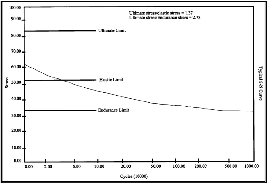
Figure description:
Typical S-N Curve
Typical S-N Curve
Legend
- S-N Curve — color: black; symbol: Solid line
- Ultimate Limit — color: black; symbol: Solid horizontal line
- Elastic Limit — color: black; symbol: Solid horizontal line
- Endurance Limit — color: black; symbol: Solid horizontal line
Annotations
- Ultimate stress/elastic stress = 1.37 (text_label - position: Top right area of the chart)
- Ultimate stress/Endurance stress = 2.78 (text_label - position: Top right area of the chart, below previous label)
- Ultimate Limit (text_label - position: y = 83.2, next to the line)
- Elastic Limit (text_label - position: y = 52.1, next to the line)
- Endurance Limit (text_label - position: y = 33.6, next to the line)
| Cycles (10000) | S-N Curve Stress | Ultimate Limit | Elastic Limit | Endurance Limit |
|---|---|---|---|---|
| 0.00 | 62.0 | 83.2 | 52.1 | 33.6 |
| 2.00 | 55.0 | 83.2 | 52.1 | 33.6 |
| 5.00 | 51.5 | 83.2 | 52.1 | 33.6 |
| 10.00 | 46.0 | 83.2 | 52.1 | 33.6 |
| 20.00 | 42.0 | 83.2 | 52.1 | 33.6 |
| 50.00 | 38.5 | 83.2 | 52.1 | 33.6 |
| 100.00 | 37.0 | 83.2 | 52.1 | 33.6 |
| 200.00 | 36.0 | 83.2 | 52.1 | 33.6 |
| 500.00 | 34.0 | 83.2 | 52.1 | 33.6 |
| 1000.00 | 33.5 | 83.2 | 52.1 | 33.6 |
Notes: The x-axis represents 'Cycles (10000' on a logarithmic scale, while the y-axis represents 'Stress' on a linear scale. Note that the textual ratios for stress limits provided at the top right show some discrepancy with the visual positions of the horizontal limit lines.)
Figure 515.8F-6. Typical S/N curve.
Exaggeration factors for materials whose fatigue characteristics are unknown or for failure mechanisms other than fatigue (such as loosening of threaded connections) cannot be calculated. However, when considering the wide range of dynamic forcing functions considered over the life cycle of most hardware, test durations calculated using Miner's rule have proven to be generally acceptable regardless of the failure mechanism under consideration.
Miner's rule, as with any analysis method, is not without its shortcomings. The text "Shock and Vibration Handbook", fourth Edition, C Harris, 1996, identifies two shortcomings. In reference to Miner's rule the text states, "... it does not consider the sequence of loading and assumes that damage in any individual stress cycle is independent of what has preceded it. Furthermore, it assumes that damage accumulation is independent of stress amplitude.” However, the same text refers to Miner's rule as "the most commonly applied linear damage rule". Its acceptance in the vibration community certainly supports Harris's assertion. The use of Miner's rule for VSD is recommended by many national and international documents. However, care should be taken to assure that Miner's rule is applied properly and with an understanding of its limitations.