Method 517.3 method · MIL-STD-810H

517.3 PYROSHOCK CONTENTS

Paragraph		Page
1.	SCOPE	1
1.1	PURPOSE	1
1.2	APPLICATION	1
1.2.1	PYROSHOCK	1
1.2.2	PYROSHOCK - MOMENTUM EXCHANGE	2
1.2.3	PYROSHOCK - PHYSICAL PHENOMENON	2
1.2.4	CLASSIFICATION OF PYROSHOCK ZONES	2
1.3	LIMITATIONS	3
2.	TAILORING GUIDANCE	3
2.1	SELECTING THE PYROSHOCK METHOD	3
2.1.1	EFFECTS OF PYROSHOCK	3
2.1.2	SEQUENCE AMONG OTHER METHODS	4
2.2	SELECTING A PROCEDURE	4
2.2.1	PROCEDURE SELECTION CONSIDERATIONS	4
2.2.2	DIFFERENCE AMONG PROCEDURES	5
2.3	DETERMINE TEST LEVELS AND CONDITIONS	5
2.3.1	GENERAL CONSIDERATIONS - TERMINOLOGY	5
2.3.2	SINGLE PYROSHOCK EVENT MEASUREMENT SYSTEM CHARACTERIZATION AND BASIC PROCESSING	11
2.3.3	TEST CONDITIONS - SHOCK SPECTRUM TRANSIENT DURATION AND SCALING	14
2.3.3.1	PYROSHOCK SOURCE ENERGY SCALING (SES)	14
2.3.3.2	PYROSHOCK RESPONSE LOCATION DISTANCE SCALING (RLDS)	14
2.3.3.3	MEASURED DATA AVAILABLE FROM PYROSHOCK	15
2.3.3.4	MEASURED DATA NOT AVAILABLE FROM PYROSHOCK	16
2.3.4	TEST AXES, DURATION, AND NUMBER OF SHOCK EVENTS	18
2.3.4.1	GENERAL	18
2.3.4.2	PROCEDURE I - NEAR-FIELD WITH AN ACTUAL CONFIGURATION	18
2.3.4.3	PROCEDURE II - NEAR-FIELD WITH A SIMULATED CONFIGURATION	18
2.3.4.4	PROCEDURE III-MID-FIELD WITH A MECHANICAL TEST DEVICE	19
2.3.4.5	PROCEDURE IV - FAR-FIELD WITH A MECHANICAL TEST DEVICE	19
2.3.4.6	PROCEDURE V - FAR-FIELD WITH AN ELECTRODYNAMIC SHAKER	19
2.4	TEST ITEM CONFIGURATION	19
3.	INFORMATION REQUIRED	19
3.1	PRETEST	19
3.2	DURING TEST	20
3.3	POST-TEST	20
4.	TEST PROCESS	20
4.1	TEST FACILITY	20
4.2	CONTROLS	21
4.2.1	CALIBRATION	21
4.2.2	TOLERANCES	21

MIL-STD-810H

METHOD 517.3

CONTENTS - Continued

Paragraph		Page
4.2.2.1	PROCEDURE I - NEAR-FIELD WITH AN ACTUAL CONFIGURATION AND PROCEDURE II - NEAR-FIELD WITH A SIMULATED CONFIGURATION	21
4.2.2.2	PROCEDURE III-MID-FIELD WITH A MECHANICAL TEST DEVICE	21
4.2.2.3	PROCEDURE IV - FAR-FIELD WITH A MECHANICAL TEST DEVICE	22
4.2.2.4	PROCEDURE V - FAR-FIELD WITH AN ELECTRODYNAMIC SHAKER	22
4.2.3	INSTRUMENTATION	22
4.2.4	DATA ANALYSIS	24
4.3	TEST INTERRUPTION	24
4.3.1	INTERRUPTION DUE TO LABORATORY EQUIPMENT MALFUNCTION	24
4.3.2	INTERRUPTION DUE TO TEST ITEM OPERATION FAILURE	24
4.4	TEST EXECUTION	25
4.4.1	PREPARATION FOR TEST	25
4.4.1.1	PRELIMINARY STEPS	25
4.4.1.2	PRETEST CHECKOUT	25
4.4.2	TEST PROCEDURES	25
4.4.2.1	PROCEDURE I - NEAR-FIELD WITH ACTUAL CONFIGURATION	26
4.4.2.2	PROCEDURE II - NEAR-FIELD WITH SIMULATED CONFIGURATION	26
4.4.2.3	PROCEDURE III- MID-FIELD USING MECHANICAL TEST DEVICE	26
4.4.2.4	PROCEDURE IV - FAR-FIELD USING MECHANICAL TEST DEVICE	27
4.4.2.5	PROCEDURE V-FAR-FIELD USING ELECTRODYNAMIC SHAKER	28
5.	ANALYSIS OF RESULTS	28
5.1	PROCEDURE I - NEAR-FIELD WITH AN ACTUAL CONFIGURATION	28
5.2	PROCEDURE II - NEAR-FIELD WITH SIMULATED CONFIGURATION	28
5.3	PROCEDURE III - MID-FIELD USING MECHANICAL TEST DEVICE	28
5.4	PROCEDURE IV - FAR-FIELD USING MECHANICAL TEST DEVICE	29
5.5	PROCEDURE V - FAR-FIELD USING ELECTRODYNAMIC SHAKER	29
6.	REFERENCE/RELATED DOCUMENTS	29
6.1	REFERENCED DOCUMENTS	29
6.2	RELATED DOCUMENTS	30

FIGURES

FIGURE 517.3-1	FULL DURATION NEAR-FIELD, LASER PYROSHOCK TIME HISTORY (MEAN REMOVED, FILTERED AT 200 KHz).	6
FIGURE 517.3-2	FULL DURATION NEAR-FIELD, LASER PYROSHOCK VELOCITY TIME HISTORY	7
FIGURE 517.3-3	FULL DURATION NEAR-FIELD, ACCELEROMETER PYROSHOCK TIME HISTORY	8
FIGURE 517.3-4	FULL DURATION NEAR-FIELD, ACCELEROMETER PYROSHOCK VELOCITY TIME HISTORY	8
FIGURE 517.3-5	ACCELERATION MAXIMAX SRS FOR THE PYROSHOCK, PRE-PYROSHOCK, AND POST PYROSHOCK (LASER).	9
FIGURE 517.3-6	MAXIMAX PSEUDO-VELOCITY RESPONSE SPECTRUM FOR THE PYROSHOCK (LASER)	10
FIGURE 517.3-7	FILTER ATTENUATION (CONCEPTUAL, NOT FILTER SPECIFIC)	12
FIGURE 517.3-8	ILLUSTRATION OF SAMPLING RATES AND OUT OF BAND "FOLD OVER” FREQUENCIES FOR DATA ACQUISITION SYSTEMS.	13
FIGURE 517.3-9	EMPIRICAL SCALING RELATIONSHIP FOR SHOCK RESPONSE SPECTRUM AS A FUNCTION OF THE DISTANCE FROM THE PYROTECHNIC SOURCE	15
FIGURE 517.3-10	SHOCK RESPONSE SPECTRA FOR VARIOUS POINT SOURCE PYROTECHNIC DEVICES	17
FIGURE 517.3-11	SHOCK RESPONSE SPECTRUM VERSUS DISTANCE FROM PYROTECHNIC SOURCE	17
FIGURE 517.3-12	PEAK PYROSHOCK RESPONSE VERSUS DISTANCE FROM PYROTECHNIC SOURCE	18

MIL-STD-810H

METHOD 517.3

CONTENTS - Continued Paragraph

Page

METHOD

517.3 ANNEX A

GUIDELINES FOR ADDITIONAL PYROSHOCK TIME HISTORY VALIDATION AND PROCESSING

1.	INTRODUCTION	A-1
2.	ALIASED DATA	A-1
3.	SLEW RATE CONTAMINATED DATA	A-4
4.	ACCELEROMETER DATA WITH BASE STRAIN EFFECTS	A-9

ANNEX A FIGURES

FIGURE 517.3A-1.	A NEAR-FIELD PYROSHOCK FOLLOWED BY TWO MECHANICAL SHOCK EVENTS	.A-2
FIGURE 517.3A-2.	THE INTEGRAL OF THE ACCELERATION DATA IN FIGURE 517.3A-1	A-2
FIGURE 517.3A-3.	DISCRETE FOURIER TRANSFORM OF THE DATA IN FIGURE 517.3A-1	A-3
FIGURE 517.3A-4.	THE SHOCK RESPONSE SPECTRA OF THE ACCELERATION DATA IN FIGURE 517.3A-1 (Q=10).	.A-3
FIGURE 517.3A-5.	A NEAR-FIELD PYROSHOCK ACCELERATION TIME HISTORY	.A-4
FIGURE 517.3A-6.	THE INTEGRAL OF THE ACCELERATION DATA IN FIGURE 517.3A-5	.A-5
FIGURE 517.3A-7.	DISCRETE FOURIER TRANSFORM OF THE DATA IN FIGURE 517.3A-5	.A-6
FIGURE 517.3A-8.	SHOCK RESPONSE SPECTRUM OF THE ACCELERATION TIME HISTORY FIGURE 517.3A-5 (Q=10)	A-6
FIGURE 517.3A-9.	TIME HISTORY OF WAVELET CORRECTION REMOVED FROM THE ACCELERATION TIME HISTORY IN FIGURE 517.3A-5	.A-7
FIGURE 517.3A-10.	SHOCK RESPONSE SPECTRUM COMPARISON FOR CORRUPTED ACCELERATION (FIGURE 517.3A-5) AND REMOVED WAVELET CORRECT (FIGURE 517.3A-9) (Q=10)	.A-7
FIGURE 517.3A-11.	SHOCK RESPONSE SPECTRUM CALCULATED FOR THE WAVELET CORRECTED ACCELERATION TIME HISTORY (Q=10)	A-8
FIGURE 517.3A-12.	A NEAR-FIELD PYROSHOCK ACCELERATION TIME HISTORY	.A-8
FIGURE 517.3A-13.	THE INTEGRAL OF THE ACCELERATION DATA IN FIGURE 517.3A-12	.A-9
FIGURE 517.3A-14.	A NEAR-FIELD PYROSHOCK ACCELERATION TIME HISTORY	A-10
FIGURE 517.3A-15.	THE INTEGRAL OF THE ACCELERATION DATA IN FIGURE 517.3A-14	A-10

Downloaded from https://www.everyspec.com

MIL-STD-810H METHOD 517.3

(This page is intentionally blank.)

MIL-STD-810H METHOD 517.3

METHOD

517.3 PYROSHOCK

NOTE: Tailoring is essential. Select methods, procedures, and parameter levels based on the tailoring process described in Part One, paragraph 4.2.2, and Annex C. Apply the general guidelines for laboratory test methods described in Part One, paragraph 5 of this Standard.

517.3 ANNEX A METHOD 517.3, ANNEX A GUIDELINES FOR ADDITIONAL PYROSHOCK TIME HISTORY VALIDATION AND PROCESSING

517.3 ANNEX A

Acceleration vs Time | Time

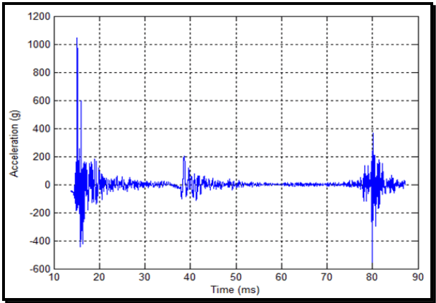
Figure description:

Acceleration vs Time

Time (ms)	Acceleration (g)
13.5	-45
14.5	-90
15.0	1050
15.3	-180
15.8	600
16.2	-440
17.5	160
18.5	-150
20.0	50
25.0	15
30.0	-10
35.0	5
38.0	-100
38.8	200
40.0	-100
41.5	110
42.5	-110
50.0	0
60.0	0
70.0	0
78.5	-120
79.5	140
80.1	-600
80.3	410
81.0	-280
81.5	210
82.5	-180
84.0	50
87.0	0

Notes: The chart shows a signal with three distinct bursts of acceleration over time. The first burst occurs around 15 ms with a peak magnitude of over 1000g. A second, smaller burst occurs near 40 ms, and a third significant burst occurs around 80 ms, including the overall minimum acceleration value of approximately -600g.

Figure 517.3A-1. A near-field pyroshock followed by two mechanical shock events.

Velocity over Time Velocity vs

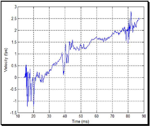
Figure description:

Velocity over Time

Velocity vs. Time

Time (ms)	Velocity (fps)
13.5	0.0
14.5	0.2
15.0	0.5
15.5	-0.4
16.0	-1.2
17.0	-0.2
18.0	-1.0
19.0	-0.5
20.0	-1.2
21.0	-0.1
22.5	0.2
24.0	0.0
25.5	-0.2
27.0	0.1
30.0	0.3
33.0	0.6
35.0	0.7
38.0	1.0
39.0	0.2
40.0	0.5
41.0	1.4
42.0	0.6
43.0	1.5
45.0	1.3
48.0	1.2
50.0	1.4
53.0	1.2
55.0	1.4
58.0	1.6
60.0	1.7
63.0	1.6
66.0	1.6
68.0	1.7
70.0	1.8
73.0	1.9
75.0	2.0
78.0	2.1
79.0	1.5
80.0	2.2
81.0	2.0
82.0	2.8
84.0	2.1
86.0	2.4
88.0	2.5

Notes: The data values are estimated based on the grid lines and axes provided in the image. The plot shows high-frequency noise or oscillation especially between 14-22 ms and 38-44 ms and 78-84 ms.

Figure 517.3A-2. The integral of the acceleration data in Figure 517.3A-1.

The discrete Fourier transform in Figure 517.3A-3 shows additional verification of the aliasing problem. An anti- aliasing filter with 60 dB/octave attenuation has 10 decade/decade slope on a log-log plot. Clearly the discrete Fourier transform in Figure 517.3A-3 does not have this attenuation and even starts to increase as it approaches the Nyquist frequency, an additional indication of aliasing. The positive and negative shock response spectra (SRS) are shown in Figure 517.3A-4.

MIL-STD-810H METHOD 517.3 ANNEX A

Magnitude

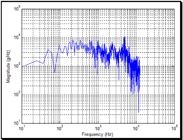
Figure description:

Magnitude (g/Hz vs Frequency (Hz

Frequency (Hz)	Magnitude (g/Hz)
10	1000
25	1500
40	1200
50	3500
70	600
100	5000
200	8500
400	6000
700	4000
1000	4500
2000	6500
4000	4000
5000	10000
8000	2000
10000	1500
11000	800
12000	2000
13000	25

Notes: The chart is a log-log plot showing a noisy signal representing Magnitude (g/Hz versus Frequency (Hz. The frequency axis ranges from 10^1 to 10^5 Hz, and the magnitude axis ranges from 10^1 to 10^5 g/Hz. The data series is represented by a single blue line. The values in the table are approximate representative points taken from the plot's logarithmic grid.))

Figure 517.3A-3. Discrete Fourier transform of the data in Figure 517.3A-1.

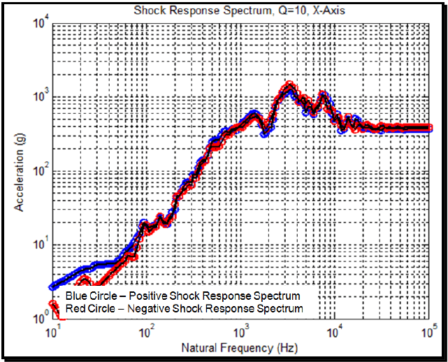
Shock Response Spectrum Q=10, X-Axis Shock Response Spectrum, Q=10, X-Axis Legend

Figure description:

Shock Response Spectrum Q=10, X-Axis

Shock Response Spectrum, Q=10, X-Axis

Legend

Positive Shock Response Spectrum — color: blue; symbol: Blue Circle
Negative Shock Response Spectrum — color: red; symbol: Red Circle

Natural Frequency (Hz)	Positive Shock Response Spectrum (g)	Negative Shock Response Spectrum (g)
10	2.5	1.8
15	4.2	2.6
20	5.2	3.5
30	5.5	2.8
40	6.0	4.5
50	8.0	6.0
70	13	7.5
80	20	10
100	18	15
150	25	20
200	45	40
300	90	75
500	260	210
1000	580	520
1500	620	550
2000	380	450
3500	1500	1700
5000	950	850
7500	1200	1150
10000	650	550
15000	520	420
20000	450	430
30000	420	410
50000	400	400
100000	400	400

Notes: The chart is a log-log plot showing acceleration (g versus natural frequency (Hz. Both the positive and negative shock response spectrums converge to approximately 400g at frequencies above 20 kHz.))

Figure 517.3A-4. The shock response spectra of the acceleration data in Figure 517.3A-1 (Q=10).

These two SRS are plausible, especially if the SRS is not plotted below 100 Hz. Additionally, the positive and negative SRS show agreement that indicates good pyroshock data. In summary, the problems with these data are: inadequate sample rate, inadequate anti-aliasing filter, and inadequate zero time before and after the complex shock. The problems can be assessed by an inspection of the accelerometer and DAS specifications. However, these are problems that cannot be detected by examination of the acceleration time history and the SRS alone and emphasize the importance of integrating the acceleration time history as per paragraph 6.1, references b and d.

MIL-STD-810H METHOD

517.3 ANNEX A

a high degree of confidence because the low-frequency asymptote is correct and the high-frequency content has been preserved. The positive and negative SRS in Figure 517.3A-11 show good agreement typical of a pyroshock or a pyroshock simulation. More details concerning the data analysis are in paragraph 6.1, reference q.

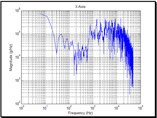
Spectral Analysis Magnitude X-Axis | Frequency

Figure description:

Spectral Analysis Magnitude

X-Axis

Frequency (Hz)	Magnitude (g/Hz)
6	720000
10	600000
15	250000
20	100000
30	15000
45	95000
60	40000
80	62000
100	25000
150	48000
180	1800
200	15000
300	25000
400	12000
600	28000
800	220000
1000	85000
1500	410000
2000	320000
3000	450000
5000	380000
8000	420000
10000	210000
15000	350000
20000	180000
30000	65000
40000	25000
50000	450

Notes: The chart is a log-log plot showing Magnitude (g/Hz versus Frequency (Hz. The data is highly variable at frequencies above 800 Hz, representing a complex spectrum. Data points in the markdown table are sampled approximations from the visual plot.))

Figure 517.3A-7. Discrete Fourier transform of the data in Figure 517.3A-5.

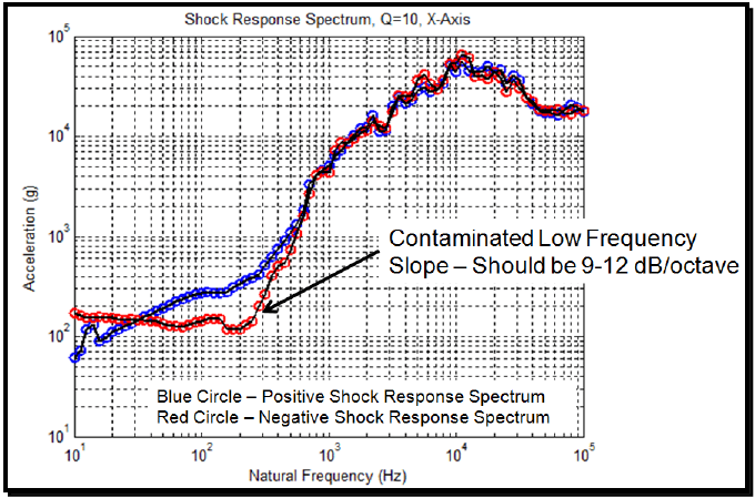
Shock Response Spectrum, Q=10, X-Axis Shock Response Spectrum, Q=10, X-Axis Legend

Figure description:

Shock Response Spectrum, Q=10, X-Axis

Shock Response Spectrum, Q=10, X-Axis

Legend

Positive Shock Response Spectrum — color: blue; symbol: Blue Circle
Negative Shock Response Spectrum — color: red; symbol: Red Circle

Annotations

Contaminated Low Frequency Slope – Should be 9-12 dB/octave (text_label - position: Natural Frequency (Hz ≈ 300, Negative Shock Response Spectrum))

Natural Frequency (Hz)	Positive Shock Response Spectrum (g)	Negative Shock Response Spectrum (g)
10	60	180
12	80	160
15	100	160
20	130	160
30	160	160
40	190	150
60	230	140
80	260	130
100	280	160
150	350	120
200	450	120
250	600	220
300	800	450
400	1200	1000
500	2000	1800
600	3000	2800
800	5000	4500
1000	7500	7000
1500	11000	11000
2000	15000	13000
2500	21000	21000
3000	30000	28000
4000	35000	35000
5000	45000	40000
6000	35000	32000
7000	40000	45000
8000	55000	50000
10000	75000	65000
12000	55000	50000
15000	50000	45000
20000	45000	40000
25000	55000	50000
30000	40000	45000
40000	25000	25000
50000	20000	20000
60000	18000	18000
80000	20000	20000
100000	18000	18000

Notes: The chart represents a Shock Response Spectrum with a quality factor (Q of 10 for the X-axis. Both the Natural Frequency (Hz on the x-axis and the Acceleration (g on the y-axis are plotted on logarithmic scales. An annotation points to an area of the negative spectrum that may be contaminated by low-frequency noise.)))

Figure 517.3A-8. Shock response spectrum of the acceleration time history in Figure 517.3A-5 (Q=10).

MIL-STD-810H METHOD 517.3 ANNEX A

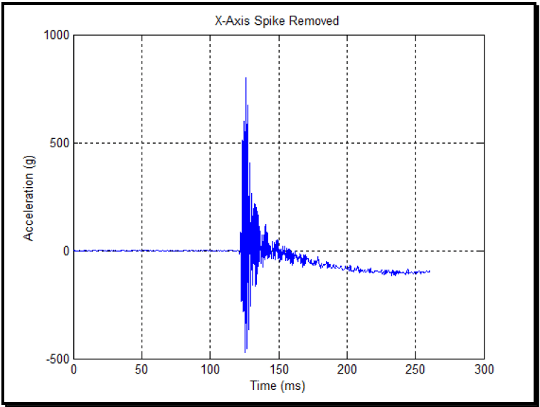
X-Axis Spike Removed X-Axis Spike Removed | Time

Figure description:

X-Axis Spike Removed

X-Axis Spike Removed

Time (ms)	Acceleration (g)
0	0
25	0
50	0
75	0
100	0
110	0
115	0
120	0
121	100
123	550
125	800
126	-480
128	680
130	100
132	210
135	230
140	180
145	90
150	30
160	-10
170	-35
180	-60
190	-75
200	-85
225	-95
250	-105
260	-100

Notes: The plot shows an acceleration event occurring around 122ms. There is a sharp spike reaching approximately 800g and dropping to nearly -500g, followed by high-frequency oscillations that decay into a steady-state value of roughly -100g by 250ms.

Figure 517.3A-9. Time history of wavelet correction removed from the acceleration time history in Figure 517.3A-5.

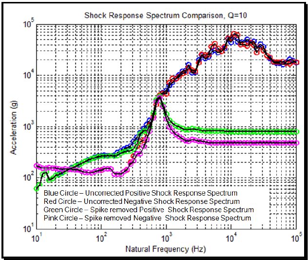
Shock Response Spectrum Comparison, Q=10 Shock Response Spectrum Comparison, Q=10 Legend

Figure description:

Shock Response Spectrum Comparison, Q=10

Shock Response Spectrum Comparison, Q=10

Legend

Uncorrected Positive Shock Response Spectrum — color: blue; symbol: Blue Circle
Uncorrected Negative Shock Response Spectrum — color: red; symbol: Red Circle
Spike removed Positive Shock Response Spectrum — color: green; symbol: Green Circle
Spike removed Negative Shock Response Spectrum — color: pink; symbol: Pink Circle

Natural Frequency (Hz)	Uncorrected Positive (g)	Uncorrected Negative (g)	Spike removed Positive (g)	Spike removed Negative (g)
10	70	70	60	180
20	120	110	110	150
50	180	180	180	160
100	250	250	250	250
200	380	350	380	130
300	450	400	450	200
400	750	650	750	550
500	1000	850	1000	1200
700	3500	3500	3500	3500
1000	5000	5000	1500	1300
1500	10000	9000	1100	800
2000	12000	11000	1000	600
3000	20000	18000	950	550
5000	30000	35000	900	500
10000	55000	60000	850	500
20000	45000	38000	850	500
50000	18000	18000	850	500
100000	18000	18000	850	500

Notes: The chart uses logarithmic scales for both axes. 'g' refers to the acceleration due to gravity.

Figure 517.3A-10. Shock response spectrum comparison for corrupted acceleration (Figure 517.3A-5) and removed wavelet correct (Figure 517.3A-9) (Q=10).

MIL-STD-810H METHOD 517.3 ANNEX A

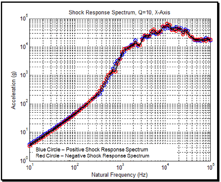
Shock Response Spectrum, Q=10, X-Axis Shock Response Spectrum, Q=10, X-Axis Legend

Figure description:

Shock Response Spectrum, Q=10, X-Axis

Shock Response Spectrum, Q=10, X-Axis

Legend

Positive Shock Response Spectrum — color: blue; symbol: Circle
Negative Shock Response Spectrum — color: red; symbol: Circle

Natural Frequency (Hz)	Positive Shock Response Spectrum (g)	Negative Shock Response Spectrum (g)
10	3.8	3.2
15	6.0	5.5
20	8.5	7.5
30	14.0	12.0
50	28.0	24.0
70	45.0	40.0
100	70.0	65.0
150	130.0	115.0
200	200.0	180.0
300	350.0	300.0
500	850.0	950.0
700	1500.0	1300.0
1000	4500.0	3800.0
1500	9000.0	8500.0
2000	17000.0	12000.0
3000	25000.0	22000.0
5000	42000.0	38000.0
7000	45000.0	48000.0
10000	55000.0	68000.0
15000	50000.0	45000.0
20000	40000.0	35000.0
30000	45000.0	40000.0
40000	30000.0	25000.0
50000	22000.0	24000.0
70000	19000.0	20000.0
100000	18000.0	18000.0

Notes: The chart is a log-log plot showing acceleration (g versus natural frequency (Hz. Q factor is 10 and data is for the X-Axis. Data points are estimated based on the logarithmic grid lines.))

Figure 517.3A-11. Shock response spectrum calculated for the wavelet corrected acceleration time history. (Q-10).

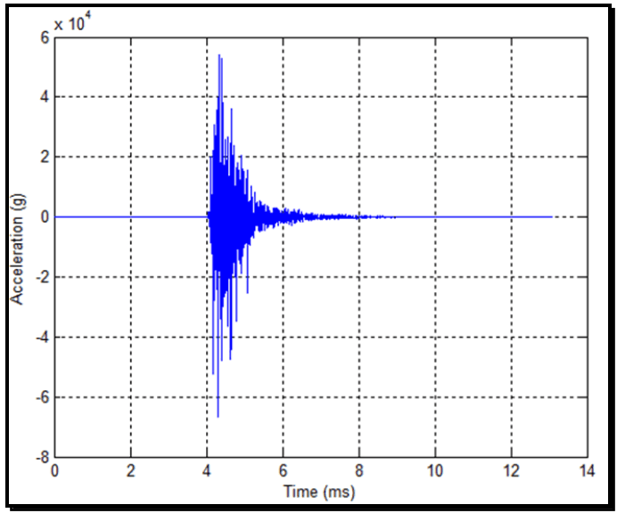
High-Frequency Acceleration Transient Acceleration vs

Figure description:

High-Frequency Acceleration Transient

Acceleration vs. Time

Time (ms)	Acceleration (g)
0.0	0
1.0	0
2.0	0
3.0	0
3.9	0
4.0	5000
4.1	-35000
4.2	45000
4.3	-68000
4.4	54000
4.5	-45000
4.7	25000
5.0	-18000
5.2	10000
5.5	-5000
6.0	3000
7.0	-1000
8.0	500
9.0	0
10.0	0
11.0	0
12.0	0
13.0	0

Notes: The y-axis units are scaled by 10^4 as indicated by the 'x 10^4' notation above the axis. The acceleration signal shows a high-frequency transient event starting at approximately 4.0 ms, reaching peak values of approximately 5.4 x 10^4 g and -6.8 x 10^4 g before decaying to near-zero by 8.0 ms.

Figure 517.3A-12. A near-field pyroshock acceleration time history.

517.3Method 517.3 method

517.3 PYROSHOCK CONTENTS

MIL-STD-810H

CONTENTS - Continued

FIGURES

MIL-STD-810H

CONTENTS - Continued Paragraph

METHOD

517.3 ANNEX A

ANNEX A FIGURES

METHOD

517.3 PYROSHOCK

517.3 ANNEX A METHOD 517.3, ANNEX A GUIDELINES FOR ADDITIONAL PYROSHOCK TIME HISTORY VALIDATION AND PROCESSING

517.3 ANNEX A

MIL-STD-810H METHOD

517.3 ANNEX A

517.3 ANNEX A

MIL-STD-810H METHOD

517.3 ANNEX A

517.3Method 517.3 method

517.3 PYROSHOCK CONTENTS

MIL-STD-810H

CONTENTS - Continued

FIGURES

MIL-STD-810H

CONTENTS - Continued Paragraph

METHOD

517.3 ANNEX A

ANNEX A FIGURES

METHOD

517.3 PYROSHOCK

517.3 ANNEX A METHOD 517.3, ANNEX A GUIDELINES FOR ADDITIONAL PYROSHOCK TIME HISTORY VALIDATION AND PROCESSING

517.3 ANNEX A

MIL-STD-810H METHOD

517.3 ANNEX A

517.3 ANNEX A

MIL-STD-810H METHOD

517.3 ANNEX A