The following minimal information is required to conduct and document dynamic tests adequately. Tailor the lists to the specific circumstances, adding or deleting items as necessary. Performing fixture and materiel modal surveys is highly recommended. These data are useful in evaluating test results, and in evaluating the suitability of materiel against changing requirements or for new applications. These data can be particularly valuable in future programs where the major emphasis will be to use existing materiel in new applications. (When modal survey is ruled out for programmatic reasons, a simple resonance search can sometimes provide useful information).
527.2-3 CONTROL IMPLEMENTATION
It is not the intent of this document to provide the specifics of the control algorithms used in the conduct of MESA and MEMA vibration testing. In fact, the various MET control system vendors do not always approach control in the same manner. There are, however, a few basic concepts that are keys to the MESA and MEMA control problem that will be addressed in the following sections.
The theory relative to linear accelerometer placement discussed in Annex A was developed from a time domain perspective. While the time domain approach is very useful in developing an understanding of the basic rigid body kinematics leading to establishing requirements for mapping of acceleration to an arbitrary point (i.e., a drive point), it is not practical to implement as a real time control scheme. In practice, the drive files are generated based on frequency-domain transfer function approximations.
Control system vendors have developed various control algorithms for conduct of a MDOF MET. Although vendors may consider the details of many of their vendor specific techniques to be proprietary, the following general discussion regarding type H transfer function estimations for a MDOF case is still relevant, and serves as a working introduction 1 to the basic control scheme. Basic definitions are reviewed to illustrate the importance of cross- spectrum components in the conduct of a MDOF MET. This discussion is summarized in this Annex and discussed in detail by Bendat and Piersol in paragraph 6.1, reference d.
527.2-3 TEST TOLERANCES FOR A PROCEDURE I MET
As discussed in paragraph 4.2.2, at this point in TWR test philosophy, test tolerance specification is not well quantified. However, numerous candidates for quantifying TWR testing are provided in the Annex section of Method 525.2. Each of the metrics addressed in Method 525.2-Annex A for SESA TWR is also applicable to the MDOF case, only the MDOF case will consist of an “array” of reference channels and an “array” of control channels. As is the case for SESA TWR, recommend the reference time histories be segmented into categories of stationary random, shock, or non-stationary, and the tolerance criteria be applied to each segment based on the data classification. For tolerance development purposes for TWR, the tolerances should not exceed the tolerances provided in Methods 514.8, 516.8, and 519.8 respectively, for stationary random vibration and mechanical shock categories. The tolerances for the third form of time trace, non-stationary data, are somewhat dependent on the nature of the non-stationarity. Techniques for non-stationarity assessment for which time trace amplitude is a function of both time and frequency are available (see paragraph 6.1, reference d). Some non-stationary time traces that have time invariant frequency characteristics can be represented by the Product Model (PM), and can be processed for tolerance purposes as stationary random vibration with a time-varying envelope. Consult Annexes A and B of Method 525.2 for details of TWR tolerance specification for non-stationary time traces. Finally, in addition to time segmenting the overall reference and control traces, it may be desirable to establish separate test tolerances over common bandwidths of the reference and control time traces, i.e., perform frequency segmenting. This could be accomplished through digital filter scheme. This Method provides no guidance for tolerance development under frequency segmentation.
527.2-3 TEST TOLERANCES FOR A PROCEDURE II MET
In general, all test tolerances need to be established based on some comparison in the frequency domain of the auto-spectral and cross-spectral density specifications with the corresponding laboratory test measured auto-spectral and cross-spectral information. Substantial reliance with respect to tolerances will be made on the auto-spectral density information, with cross-spectral density information playing a secondary role because of its reliance on measurement channel coherence for error characterization. Basic comparison might be taken for nominal test tolerances performed by the vendor-supplied MET software. Test laboratory personnel need to consult the vendor-supplied MET system manuals for such tolerances, and have a very clear understanding of the proper interpretation of the test tolerances. Unfortunately, the question of reasonable tolerances in a MET is not simple. Generally, the test tolerances prescribed in Method 514.8 for stationary random vibration are applicable for auto-spectral density information derived from a MET. However, it is often necessary to relax test tolerances on cross-spectral density information. Transfer function estimates along with coherence, partial coherence and multiple coherence function estimates may be necessary to assess the test tolerance questions. An experienced analyst will be required in cases where multi-channel measurements must be assessed for test tolerance assessment.
Since the test is run in real time, it is only necessary to ensure the reference input is properly compensated before running the test. All MET strategies and vendor software provide for very low level testing for establishing preliminary transfer function information that may be updated for higher level testing. The updated transfer function accounts for certain vibration system amplitude nonlinearities that may occur as the general level of vibration is increased.
527.2-3 REQUIRED TEST CONDITIONS
The primary function of Vibration Schedule Development (VSD) is to combine vibration measurements of numerous events that collectively represent an item’s lifetime vibration exposure (or some predefined subset thereof) into a manageable set of LVTS representing the equivalent exposure. The most dynamically accurate method to reproduce the full exposure would be to sequentially vibrate the system to all the individual, uncompressed events representing its full lifecycle. However, such an approach is generally not feasible from both schedule and economic perspectives and some compromises must be made to realize the benefits of testing in the laboratory. Time compression techniques based on fatigue equivalency are typically employed such that vibration testing can be performed in a timely and economic manner. North Atlantic Treaty Organization (NATO) Allied Environmental Conditions Test Publication (AECTP) 240, Leaflet 24103 and Method 514.8 of Mil-Std-810H, provide general guidance for developing accurate representations, and issues that should be considered during the VSD process for the SESA scenario. This Annex expands upon the discussion in Leaflet 2410 to address the general multiple exciter test scenario. Discussions will be limited to random LVTS development. At the time of this publication, no commercially available multiple-input multiple-output (MIMO) solutions exist for swept narrowband random on random (NBROR) or sine-on-random (SOR) other than Procedure I - Time Waveform Replication based techniques.
3.1 Pretest
The following information is required to adequately conduct a MET.
- a. General. Information listed in Part One, paragraphs 5.7 and 5.9 of this Standard, and in Part One, Annex A, Task 405 of this Standard.
- b. Specific to this Method.
- (1) Selection of test procedure and test system (test item/platform configuration) detailed information including:
- (a) Control sensor locations for control time traces (refer to Annex A for MET specific considerations).
- (b) Reference time histories for a Procedure I MET, or reference ASD & CSD for a Procedure II MET.
- (c) (c) Monitor/limit sensor locations (if any). ༠。 (d) (d)
- Levels of pre-test acceptable to obtain appropriate shaker system compensation.
MIL-STD-810H
METHOD 527.2
- (e) Criteria for satisfaction of the test, including previously agreed MET tolerance limits.
- (2) Ability of overall system to replicate either a measured materiel environment or an analytically specified materiel environment under a MET, including bandlimited input and the temperature effects (if any).
- c. Tailoring - Necessary variations in the basic test parameters/testing materials to accommodate Life Cycle Environmental Profile (LCEP) requirements and/or facility limitations.
527.2-3.1 SISO Auto and Cross-Spectral Definitions Review
Prior to matrix-based discussions of transfer function estimates for a MET, consider the following basic scalar definitions as presented by Bendat and Piersol in paragraph 6.1, reference d. The discussions assume two stationary (ergodic) Gaussian random processes {x(t)} and {y(t)}. The finite Fourier Transforms of {x(t)} and {y(t)} are defined as:
MIL-STD-810H
METHOD 527.2 ANNEX B
The auto and cross-spectral densities of and for an "unlimited time" length are defined respectively as:
G₁,(S)=2lim - E[|Y (ST)] T
G(S) = 2lim — E[X* (ƒ)Y(S)]
Estimates of and as computed over a "finite time" interval are defined as:
and will have a discrete spectral resolution of . Employment of and will generally be unacceptable due to the large random error associated with the "raw" estimate. In practice, the random error is reduced, (refer to paragraph 6.1, reference d, for a detailed error discussion), by computing an ensemble of different averages of length T to obtain a "smooth" estimate defined as:
3.2 SISO Transfer Function and Coherence Function Definitions Review.
Another very useful tool in the analysis of SISO linear systems are the transfer function and associated coherence estimates. Again, both concepts are explained in detail within paragraph 6.1, reference d. Using the previously defined auto and cross-spectrum definitions, the optimum frequency response function (transfer function) is defined as:
Ĥxy (ƒ)= Ĝy (f) Ĝ(ƒ)
and the associated coherence function is defined as:
Ĝ, (S) θ„ (ƒ) ¯ ¯Ĝ„(ƒ)Ĝ» (ƒ)
The transfer function provides a frequency domain view of the gain and phase relationship between the input and output signals, while the coherence function indicates the amount of causality in the transfer function. The coherence function range is 0 ≤ γ xy 2 ( ) f ≤ , with 0 representing no causality and 1 representing perfect causality. Observe that 1
MIL-STD-810H METHOD
527.2-3.1 Composite (Global) Error Discussion for Procedure I
One obvious point of concern in addressing adequacy of a 6-DOF TWR test is in a global sense. This is analogous, in the conduct of traditional SDOF testing to the practice of providing a composite control plot summarizing multiple control channel averaging or weighting schemes. For example, experience has shown that in MEMA tests in which a specific mechanical degree-of-freedom consists of a very small percentage of the composite energy across all mechanical degrees-of-freedom, the associated error for that DOF will often be higher than the desired test tolerances discussed in paragraph 3 above. Three candidates, (many others are possible) for accessing global error are addressed in paragraph 6.1, reference k, and summarized below. The three techniques discussed below are consistent with the rudimentary division of data types discussed in Method 525.2, Annex A.
527.2-3.1 Composite (Global) Error Discussion for Procedure II
The same issues discussed in Annex C, paragraph 3.1, apply to Procedure II MET. However, for a Procedure II test, the time histories synthesized by the control system will be wide sense stationary and Gaussian in nature. Therefore, the global error discussion reduces to a discussion of the ASD and CSD error. Recall from the discussion in paragraph 2.2, that ASD is given priority in the control scheme, and that the degree of CSD accuracy required will be determined largely on a test-by-test basis. Addressing global error will depend largely on the MET configuration and control transducer placement. Translational and rotational degrees of freedom may be viewed in a composite sense by averaging or weighting each transducer in a common axis, or possibly by considering the composite ASD error across all axes as suggested in Annex C, paragraph 3.3. Translational degrees of freedom are readily computed from direct accelerometer measurements, while rotational degrees of freedom may be viewed in terms of the ASD computed from either direct angular motion measurements or from estimates of rotations computed from linear accelerometers. When considering estimates of rotational degrees of freedom based on linear accelerometers, refer to the guidance and caution discussed in Annex C, paragraph 2.2.
Downloaded from https://www.everyspec.com
MIL-STD-810H METHOD 527.2 ANNEX D
(This page is intentionally blank.)
MIL-STD-810H METHOD 527.2 ANNEX E
METHOD 527.2, ANNEX E
LABORATORY VIBRATION TEST SCHEDULE DEVELOPMENT
FOR MULTI-EXCITER APPLICATIONS
527.2-3.1 Test Configurations
The MIMO random vibration test problem can refer to several configurations. One configuration is multiple exciters driving a single test item in one axis. This configuration is often used for large test items too large for a single exciter. A second configuration is the excitation of a single test item with multiple exciters in more than one axis. Linear displacements along defined directions are referred to as translation degree-of-freedom (DOF) and angular displacements along those same directions are referred to as rotation DOFs. Up to six DOFs exist for a rigid body
MIL-STD-810H METHOD
3.1.1 Basic Representation of a MIMO System
All MIMO test systems are discussed using a common description in terms of matrix equations . A simplified version of the general MIMO random vibration test problem can be generalized in Figure 1. The complete mechanical system is characterized by the power amplifiers and a system of several exciters, on which is mounted a single test article. The response of the test article is monitored by a vector of response channels (represented as {c}). Each element in the vector is typically the acceleration time history from a single accelerometer. Other types of sensors can be used, with attention paid to the nature of the measurements relative to the test item and other sensors. The power amplifiers are driven by a vector of electrical drives (represented as {d}), generated by a control system. Each element in the vector is a time history driving a single shaker. The control system monitors the response of the test item {c}, and attempts to produce drive signals {d}, such that the statistics of the control signals meet some criteria as specified in the test specifications.
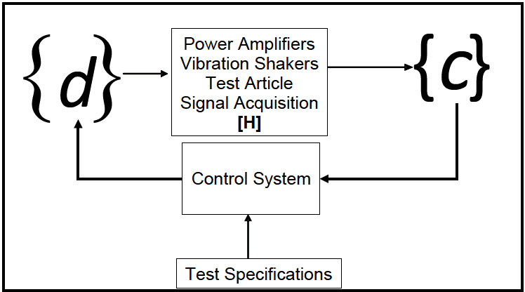
Figure description:
MDOF System Representation Entities and Information Flow:
- {d} (Drive Signals: Vector of electrical drives input to the physical system.
- Physical System [H: Comprises Power Amplifiers, Vibration Shakers, the Test Article, and Signal Acquisition.
- {c} (Response Channels: Output vector representing the monitored response (e.g., acceleration of the test article.
- Control System: Processes the response vector {c} and feedback to adjust drive signals {d}.
- Test Specifications: External input defining the criteria the control system must meet.
- Process Loop: Test Specifications → Control System → {d} → Physical System [H → {c} → feedback to Control System.
Figure 1. Basic representation of a MDOF system.
3.1.2 Generalized Representation of a MIMO System
A more generalized MIMO system is shown in Figure 2. A system under test is driven by N, shakers resulting in the response of Na control accelerometers. The accelerometer data are typically structured in blocks. Each of the acceleration records will then be a vector of time samples. Some control systems then provide for a transformation matrix, Ta, to convert the block of Na accelerometer time histories to Nc control variables. The Spectral Density Matrix (SDM) of the control variables is then estimated from the current block of data and previous data. The transformation matrix, Ta, is typically a constant independent of frequency. In theory the transformation matrix could be applied before or after the estimation of the control SDM. The estimated control SDM, C is then compared with the reference SDM, R, and a correction is computed for the drive SDM, D. The drive time histories {d} are then computed from the drive SDM, D, using time domain randomization. A second transformation matrix, Ts, is employed to transform the Na drive variables into Ns shaker drive signals. In theory, Ts could be implemented before or after the transformation into the time domain. One advantage of placing the transformation in the frequency domain section of the control algorithm is that the matrix could then be made a function of frequency. Having the transformation matrix, Ts, a constant assumes the shakers are matched and the desired transformation can be deduced.
MIL-STD-810H
METHOD 527.2 ANNEX E
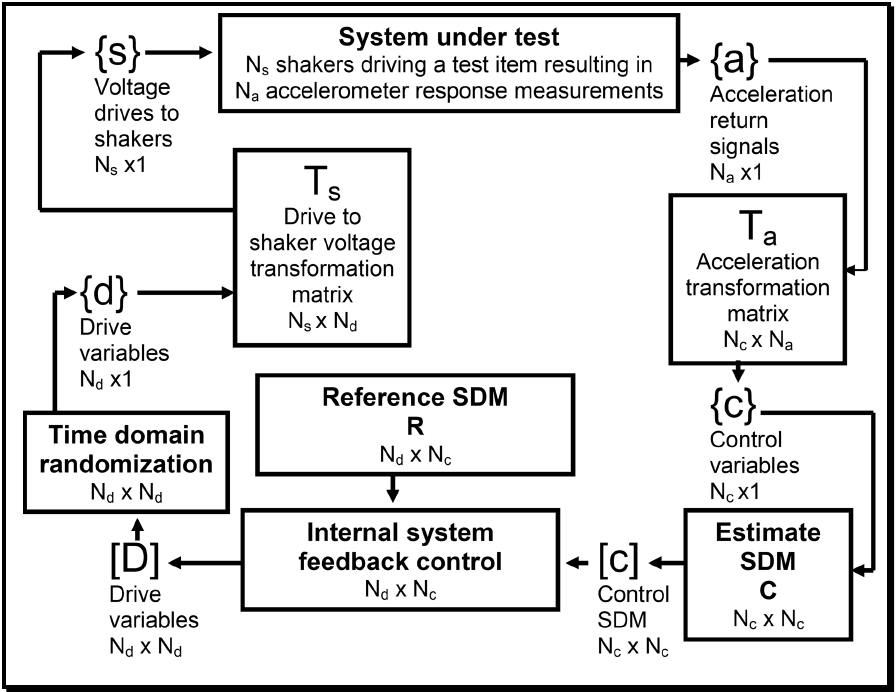
Figure description:
This image is a flowchart illustrating a control loop for a Multi-Degree-of-Freedom (MDOF system test. The key components, variables, and their relationships are detailed below.
| Component / Variable | Description | Dimensions |
|---|---|---|
| System under test | The physical item being tested, driven by Ns shakers and measured by Na accelerometers. Receives voltage \{s\} and outputs acceleration \{a\}. | - |
\{s\} | Voltage drives to shakers. | Ns x 1 |
\{a\} | Acceleration return signals from the test item. | Na x 1 |
| Ts | Drive to shaker voltage transformation matrix. Transforms drive variables \{d\} to shaker voltages \{s\}. | Ns x Nd |
| Ta | Acceleration transformation matrix. Transforms acceleration signals \{a\} to control variables \{c\}. | Nc x Na |
| Time domain randomization | Process that takes the drive variables matrix [D and outputs the drive variables vector \{d\}. | Nd x Nd |
\{d\} | Drive variables vector. | Nd x 1 |
| Estimate SDM C | Process that estimates the Control Spectral Density Matrix [C from the control variables \{c\}. | Nc x Nc |
\{c\} | Control variables vector. | Nc x 1 |
[C | Control Spectral Density Matrix (SDM, estimated from measurements.) | Nc x Nc |
| Internal system feedback control | Compares the estimated Control SDM [C with the Reference SDM R to generate the drive variables matrix [D. | Nd x Nc |
[D | Drive variables matrix. | Nd x Nd |
| R | Reference Spectral Density Matrix (SDM, representing the target state.) | Nd x Nc |
Figure 2. Generalized representation of a MDOF system.
3.2 During Test
Collect the following information while conducting the test.
- a. General. Information listed in Part One, paragraph 5.10, and in Annex A, Tasks 405 and 406 of this Standard.
- b. Specific to this Method.
- (1) Capture of the appropriately processed control time trace information in digital form for comparison with the specification. Compute key time domain engineering unit (EU) specific metrics such as rms versus time and key spectral metrics such as auto-spectral and cross-spectral density estimates, and ensure compliance with agreed-upon tolerances.
- (2) Capture of the appropriately processed monitor/limit time trace information in digital form.
- (3) Recording of the number of exposures and the duration of the dynamic environments.
- (4) Log of auxiliary environmental conditions such as temperature.
- (5) Log of any out of tolerance conditions relative to the control measurement points.
- (6) Log of materiel functional failure.
527.2-3.2 Global RMS Error
One of the most common time domain error metrics employed in TWR testing is simply comparisons between the reference data and laboratory data as EU-rms versus time computed over short time slices for the duration of the test. For the MDOF TWR case, the rms versus time error is easily calculated for each control channel as illustrated by Step 2 below. Also of interest would be an energy weighted view of the rms versus time error between the reference and control signals. This concept is developed in the following steps:
Step 1 The arrays and 1 shown in Equation 3.2.1 represent, respectively, the N point sampled JxN JxN reference and laboratory test data for each of the J control channels. Test-specific parameters such as sample frequency and filter settings should be tracked by the test operator. It is assumed that the time histories represented by Equation 3.2.1 will not have a bias, or that any bias has been removed during pre-processing.
ri(n) (1₁ (n)) r(n) = JxN r₂(n) : l(n) = JxN 1₂(n) n = 1,2...N; (3.2.1) \r₁(n)) (1,(n))
Step 2 The two matrices RMS _ r and RMS _ l shown in Equation 3.2.2 contain the g-rms values for each reference and laboratory test channel computed over each time segment, s. The j index, j = 1, J
MIL-STD-810H METHOD
527.2-3.2 Generalized MDOF Vibration Control Discussion
- a. A general discussion of the MDOF control process is provided for insight as to how the MDOF LVTS will serve as the reference in the control process. The purpose of the control loop is to minimize the difference between the reference and the control signals by making corrections to the drive signals. The correction can be computed in several ways. One method is to compute the drive from:
D = ZRZ'
where the system impedance matrix, Z, is updated as new information is gathered, or a modified reference spectrum, R, is computed based on the error in the return spectrum. The initial drive vector is typically computed using the above equation and the reference SDM. A drive signal error can also be computed from:
Sometimes an adaptive correction is used. Sometimes a combination of all methods is used.
- b. The transformation matrices are often called the input and output transformation matrices. One should be careful with this nomenclature because of the confusion between input and output. The input to the system under test (voltages to the power amplifiers or servo controllers) is the output of the control system. The output of the system under test (such as accelerometer measurements) is the input to the control system. Paragraphs 4.4.1 and 4.4.2 provide the nomenclature employed for input and output transformations, as they are applied within this document.
MIL-STD-810H METHOD
3.3 Post-Test
The following post-test data shall be included in the test report.
- a. General. Information listed in Part One paragraph 5.13, and in Annex A, Task 406 of this Standard.
- b. Specific to this Method.
- (1) Duration of exposure of the materiel to the dynamic MET environment.
- (2) Any data measurement anomalies, e.g., high instrumentation noise levels, loss of sensor response.
- (3) Status of the test materiel/fixture. In particular, any structural or functional failure of the test materiel/fixture.
- (4) Status of measurement system after each test.
- (5) Any changes from the original test plan.
527.2-3.3 MIMO Auto-Spectra, Cross-Spectra, and Initial Function Estimates
Consider the MIMO system described below consisting of m inputs and n outputs. Note that, for the general case, m ≠ n. (A Linear Time-Invariant (LTI) system is assumed).
x(t) yn(t) H
3.3.1 Frequency Domain Transfer Function Relationship
Develop a Frequency Domain transfer function relationship between the input and output. The following discussion is one of multiple approaches. Welch’s method, paragraph 6.1 reference o, is generally used to compute a smoothed estimate of the spectral terms in the following discussion.
- a. Define X(f) as column vector of the m input signals and Y(f) as a column vector of the n output signals.
X=
- b. Define the Transfer Function Matrix between X(f) and Y(f) as Hxy(f) such that the input precedes the output.
HH12 Hin H21 H 22 H2n Hxy
Hm Hm2 H
- c. Define the Instantaneous Power Spectra as:
| Sxx = X*X' | Instantaneous Input Auto-Spectrum (Dim: m x m) |
| Syy = Y*Y' | Instantaneous Output Auto-Spectrum (Dim: n x n) |
| Sxy = X*Y' | Instantaneous Cross-Spectrum (Dim: m x n) |
- d. Define the Cumulative Power Spectra over k averages as:
G„ ΙΣ -Sxx Cumulative Input Auto-Spectrum (Dim: mxm)
Jyy = Cumulative Output Auto-Spectrum (Dim: nxn)
GLY = ki-1xyi Cumulative Cross-Spectrum (Dim: mxn)
MIL-STD-810H
METHOD 527.2 ANNEX B
3.3.2 Key Transfer Function Derivations.
Given the definitions a. and b. above, it follows that:
H1 H21 Hml X₁ Y₂ H12 H22 Hm2 X2
Hin H2n Hmn
Re-write the input/output relationship in terms of the cumulative auto and cross spectra as defined above in paragraph 3.3.1d.
Y' = (HX) = X'H¸y X'Y' = X'X'Hy
GLY ΙΣΧΥΣ : xx]1, = i=1 = =G_HA G₁ =G_Hy G¸“G¸ =G¸¹G„H¸y G₁G=H mxm mxn mxn xy
H
In performing laboratory MET, the initial estimation of xy will be computed based on a set of uncorrelated random input signals. The desired signal, Y , will have been either measured directly, or possibly computed via a 6-DOF model based prediction, leaving X (that will represent the input to the vibration exciter) as the unknown.
Recall that Y = H, X, therefore, (H)" Y = (H¸)' H„X yielding (H¸)' Y = X. nx1 xy mx1 nx1 mxl nxm mxn
Note that for the general case in which m/n, the computation of (H.) will require a pseudo-inverse (Moore- Penrose) approximation. This computation involves a singular value decomposition (SVD) of H. Viewing the singular values provides two useful pieces of information. First, it provides information on a spectral line basis as to the rank of Hy, and second, it provides an indication as to the dynamic range of H, thereby providing insight into the potential for noise in computation of the drive files. Estimations of H via SVD techniques are more computationally intense than classical methods such as the Cholesky decomposition; however, the SVD technique is more robust and capable of addressing rectangular and singular matrices. SVD techniques also provide straight forward methods of addressing dynamic range and noise by investigating the ratio of the largest to smallest singular values.
From a Procedure II control algorithm perspective, one may be interested in computation of directly from . Recall from above that , from which the following is derived:
MIL-STD-810H
METHOD 527.2 ANNEX B
Y = H, X
Y' = (H„X) = XH‚y Y* = (HX) = H**X* YY' = (H™X)(X'H¸)
This yields:
Gy = H™GH yy
Which leads directly to:
G¸ = (H¨‚ )'G„ (H„
Paragraph 6.1, reference d, goes into considerably more detail, to include error analysis, regarding the discussion above. In addition, the various control system vendors continue to improve on the basic concepts using unique (and often proprietary) techniques to improve convergence to the reference array based on error in both time and frequency domains. The discussion above serves as an illustration through use of well defined and established analyses of the increased level of complexity associated with MDOF vibration testing. Of particular interest are that the fundamental principles are based on the assumption that the excitation system is LTI, and that the reference measurements were acquired from a kinematically consistent body. Clearly, neither assumption holds for the majority of laboratory vibration tests, even in the SESA case. The issue at hand is establishing metrics of acceptability for a MET.
3.3.3 Key Transfer Function Derivations Alternative
An alternative to the derivations in paragraphs 3.3.1 and 3.3.2, which is commonly employed in the MIMO vibration
control arena, is based on making the following minor changes in definitions within paragraph 3.3.1:
- a. Define X(f) as column vector of the m input signals and Y(f) as a column vector of the n output signals as defined in paragraph 3.3.1.
X₂ Y,
X= Y
- b. Define the Transfer Function Matrix between X(f) and Y(f) as Hyx(f) such that the output precedes the input. Recalling Hy as defined in paragraph 3.3.1, observe that Hyx = H, and that HÃ ± H… · xy ух xy
HH21 Hml H₁₂ H22 Hm2 H =
H H₂ H
nx1 Y = Hyx X nxm ух mx1
MIL-STD-810H
METHOD 527.2 ANNEX B
c. Define the Instantaneous Power Spectra as:
Φ. = ΧΧ" xx Instantaneous Input Auto-Spectrum (Dim: m x m)
yy =YY" Instantaneous Output Auto-Spectrum (Dim: nx n)
Q = YX" ух Instantaneous Cross-Spectrum (Dim: n x m)
Observe in comparison to the definitions provided in paragraph 3.3.1 that:
Ô¸=S…, ÔÂ =S'¼y, and y = xx yx
- d. Define the Cumulative Power Spectra over k averages as:
Φ xx = ΕΣ Φ ΣΦ Cumulative Input Auto-Spectrum (Dim: m x m)
Cumulative Output Auto-Spectrum (Dim: )
=- Φ Cumulative Cross-Spectrum (Dim: n x m) yx ki-1 yxi
Observe in comparison to the definitions provided in paragraph 3.3.1 that:
O₁ =G, y = Gyy, and Dyx = G yy ух
Applying the input/output relationship of an LTI system, and by making the following substitutions based on the definitions for the cumulative auto and cross spectra as defined above in paragraphs 3.3.3c and 3.3.3d yields the following:
1 1 Φ = H = H = and. yy k ki-1 vx ki-
„[H]¹ Or, by defining Z=H¼ simplifies to ❤¸ = ZO„Z“ yy
Φ ==Σ",\X”¨ = ±Σ_‚¤‚‚ׂX”¨ = H¸‚½‚ׂX”¨ = H„„ which leads to : XXX, ki-1 - 15k ki-1
= Hyx
Observe that two approaches discussed within paragraph 3.3 are very similar in structure. Selection of technique is generally one of preference or possibly computational advantage.
3.4 MIMO Coherence Functions
The concept of coherence will need to be expanded to address the MIMO case. Refer to the paragraph 6.1, references d and l, for a detailed discussion on this subject. Following, are three basic coherence definitions that apply to the MIMO case for a linear system.
3.4.1 Ordinary Coherence
The ordinary coherence function is defined as the correlation coefficient describing the linear relationship between any two single spectra. In the multiple input case, care must be taken in interpretation of ordinary coherence. It is possible that the coherence between the output and a given input may be much less than unity, even if the relationship is strictly linear due to the influence of other input signals. For a linear MIMO system, the ordinary coherence is defined as:
G Y²mn (f)=- where, Gxx G yynn
MIL-STD-810H METHOD
3.4.2 Partial Coherence
The partial coherence function is defined as the ordinary coherence between one conditioned output and another conditioned output, between one conditioned input and another conditioned input, or between one conditioned input and a conditioned output. The individual input and output signals are “conditioned” by removing the contributions from other inputs. There is a partial coherence function that exists for every input-input, output-output, and input-output combination for all permutations of conditioning.
3.4.3 Multiple Coherence
The multiple coherence function is defined as the correlation coefficient describing the linear relationship between a given output and all known inputs. A multiple coherence function exists for each output signal. The multiple coherence function provides an excellent method of evaluating the degree and relative importance of unknown contributions such as noise and nonlinearities to each output signal.
As is the case for ordinary coherence, a low multiple coherence value represents a low causality between the output signal of interest and the input signals. This information is critical in the closed loop control process in that it will influence the transfer function estimate. In fact, MDOF control systems use the multiple coherence function as a key test parameter. Specifically, the control algorithm will compute the multiple coherence for each output channel at each spectral line. Prior to updating the transfer function during a test, the multiple coherence function will be evaluated to ensure a specific threshold is achieved, (i.e. ). If the user-defined threshold has not been achieved, the transfer function for that spectral line will not be updated. Partial and multiple coherence are discussed in detail in paragraph 6.1, reference d. Underwood also provides an interesting perspective of both partial and multiple coherence in paragraph 6.1, reference 1.
3.5 Drive Signal Compensation
The previous discussions of auto and cross-spectral densities and how they are used in the computation of the system transfer function and associated coherence functions are all applied in the initial system identification phase in a MET. Subsequent to the initial system identification, the output (drive) signals are updated similar to the traditional SESA case. Although the details of each control system vendor’s algorithms will vary, there are two basic drive signal update methodologies.
The first drive signal update technique is based simply on continuous updates of the system transfer function, and is performed throughout the duration of the test to address minor system changes (paragraph 6.1, reference m). Note that for any frequencies for which the drive signals are fully correlated, corrections to the system transfer function will not be possible.
The second drive signal update technique is based on the error spectrum that is computed between the feedback spectrum and the specified reference spectrum. Typically, some fraction of the error is applied to a correction of the coupling matrix corrected during each loop. The coupling matrix is the spectral density matrix that couples the vector of white noise sources generated by the control system to achieve the desired reference spectrum.
MIL-STD-810H METHOD 527.2 ANNEX C