527.2 MULTI-EXCITER TEST CONTENTS
| Paragraph | Page | |
|---|---|---|
| 1. | SCOPE | 1 |
| 1.1 | PURPOSE | 1 |
| 1.2 | APPLICATION | 1 |
| 1.2.1 | GENERAL DISCUSSION | 1 |
| 1.2.2 | TERMINOLOGY | 2 |
| 1.3 | LIMITATIONS | 5 |
| 2. | TAILORING GUIDANCE | 5 |
| 2.1 | SELECTING THE MET METHOD | 5 |
| 2.1.1 | EFFECTS OF THE MET ENVIRONMENT | 5 |
| 2.1.2 | SEQUENCE AMONG OTHER METHODS | 6 |
| 2.2 | SELECTING A PROCEDURE | 6 |
| 2.2.1 | PROCEDURE SELECTION CONSIDERATIONS | 6 |
| 2.3 | DETERMINE TEST LEVELS AND CONDITIONS | 6 |
| 2.3.1 | LABORATORY TEST DATA INPUT | 7 |
| 2.3.1.1 | CROSS-SPECTRAL DENSITY CONSIDERATIONS | 7 |
| 2.3.1.2 | GENERAL | 7 |
| 2.3.2 | LABORATORY TEST OUTPUT | 7 |
| 2.4 | TEST ITEM OPERATION | 7 |
| 3. | INFORMATION REQUIRED | 7 |
| 3.1 | PRETEST | 7 |
| 3.2 | DURING TEST | 8 |
| 3.3 | POST-TEST | 8 |
| 4. | TEST PROCESS | 8 |
| 4.1 | TEST FACILITY | 8 |
| 4.2 | CONTROLS | 8 |
| 4.2.1 | CALIBRATION | 9 |
| 4.2.2 | TOLERANCES | 9 |
| 4.3 | TEST INTERRUPTION | 9 |
| 4.3.1 | INTERRUPTION DUE TO LABORATORY EQUIPMENT MALFUNCTION | 9 |
| 4.3.2 | INTERRUPTION DUE TO TEST ITEM OPERATION FAILURE | 9 |
| 4.3.3 | INTERRUPTION DUE TO A SCHEDULED EVENT | 10 |
| 4.3.4 | INTERRUPTION DUE TO EXCEEDING TEST TOLERANCES | 10 |
| 4.4 | TEST SETUP | 10 |
| 4.4.1 | INSTRUMENTATION | 10 |
| 4.4.2 | PLATFORM INTEGRATION | 11 |
| 4.4.3 | SETUP ANALYSIS | 11 |
| 4.5 | TEST EXECUTION | 11 |
| 4.5.1 | PREPARATION FOR TEST | 11 |
| 4.5.1.1 | PRELIMINARY STEPS | 12 |
| 4.5.1.2 | PRETEST STANDARD AMBIENT CHECKOUT | 12 |
| 4.5.2 | PROCEDURE | 12 |
MIL-STD-810H METHOD
527.2 CONTENTS-Continued
| Paragraph | Page | |
|---|---|---|
| 5. | ANALYSIS OF RESULTS | 13 |
| 5.1 | PHYSICS OF FAILURE | 14 |
| 5.2 | QUALIFICATION TESTS | 14 |
| 5.3 | OTHER TESTS | 14 |
| 6. | REFERENCE/RELATED DOCUMENTS | 14 |
| 6.1 | REFERENCED DOCUMENTS | 14 |
| 6.2 | RELATED DOCUMENTS | 15 |
FIGURES
| FIGURE 527.2-1. | SESA - SINGLE EXCITER VERTICAL AXIS TEST SETUP | 3 |
| FIGURE 527.2-2. | MESA (IF CONTROL CONFIGURED FOR TWO EXCITER 1-DOF MOTION) OR MEMA (IF CONTROL AND MECHANICAL COUPLINGS CONFIGURED FOR TWO EXCITER 2-DOF MOTION) | 3 |
| FIGURE 527.2-3. | MEMA - TRI-AXIAL EXCITER TEST SETUP (TRANSLATIONAL DEGREES-OF-FREEDOM) | 4 |
METHOD
527.2 ANNEX A
ENGINEERING INFORMATION FOR MET TRANSDUCER PLACEMENT
| 1. | GENERAL PHILOSOPHY FOR A MET | A-1 |
| 2. | REFERENCE POINT CONSIDERATIONS FOR MDOF TESTING | A-1 |
| 2.1 | REFERENCE DATA CONSIDERATIONS | A-1 |
| 2.2 | REFERENCE POINT KENMATICS | A-1 |
A FIGURE
FIGURE 527.2A-1. BODY WITH n ACCELEROMETERS. PLACEMENTS.. .A-2
METHOD
527.2 ANNEX B
SYSTEM IDENTIFICATION FOR LINEAR TIME-INVARIANT MDOF SYSTEMS
| 1. | TRANSFER-FUNCTION ESTIMATIONS | B-1 |
| 2. | SIGNAL TRANSFORMATION | B-1 |
| 3. | CONTROL IMPLEMENTATION | B-1 |
| 3.1 | SISO AUTO AND CROSS-SPECTRAL DEFINITIONS REVIEW | B-1 |
| 3.2 | SISO TRANSFER FUNCTION AND COHERENCE FUNCTION DEFINITIONS REVIEW | B-2 |
| 3.3 | MIMO AUTO-SPECTRA, CROSS-SPECTRA, AND INITIAL FUNCTION ESTIMATES | B-3 |
| 3.3.1 | FREQUENCY DOMAIN TRANSFER FUNCTION RELATIONSHIP | B-3 |
| 3.3.2 | KEY TRANSFER FUNCTION DERIVATIONS | B-4 |
| 3.3.3 | KEY TRANSFER FUNCTION DERIVATIONS ALTERNATIVE | B-5 |
| 3.4 | MIMO COHERENCE FUNCTIONS | B-6 |
| 3.4.1 | ORDINARY COHERENCE | B-6 |
| 3.4.2 | PARTIAL COHERENCE | B-7 |
| 3.4.3 | MULTIPLE COHERENCE | B-7 |
| 3.5 | DRIVE SIGNAL COMPENSATION | B-7 |
MIL-STD-810H
METHOD 527.2
CONTENTS-Continued
| METHOD 527.2 ANNEX C PROCEDURE I MET (TIME WAVEFORM REPLICATION (TWR) SPECIFIC) | ||
| 1. | PROCEDURE I MET (TIME DOMAIN REFERENCE CRITERIA) | .C-1 |
| 1.1 | PREPROCESSING. | C-1 |
| 2. | ANALYSIS CONSIDERATIONS FOR A PROCEDURE I MET | C-1 |
| 2.1 | ADDRESSING TRANSLATIONAL MOTION. | C-1 |
| 2.2 | ADDRESSING ANGULAR MOTION. | C-1 |
| 3. | TEST TOLERANCES FOR A PROCEDURE I MET | C-2 |
| 3.1 | COMPOSITE (GLOBAL) ERROR DISCUSSION FOR PROCEDURE I | C-2 |
| 3.2 | GLOBAL RMS ERROR | C-2 |
| 3.3 | GLOBAL ASD ERROR.. | C-4 |
| 3.4 | GLOBAL SRS ERROR | C-6 |
| METHOD 527.2 ANNEX D PROCEDURE II MET (SPECTRAL DENSITY MATRIX (SDM) SPECIFIC) | ||
| 1. | PROCEDURE II MET (FREQUENCY DOMAIN REFERENCE CRITERIA) | .D-1 |
| 1.1 | PREPROCESSING. | .D-1 |
| 2. | ANALYSIS CONSIDERATIONS FOR A PROCEDURE II MET. | .D-1 |
| 2.1 | MESA AND MEMA SPECIFICATION PARAMETERS. | D-1 |
| 2.1.1 | CROSS SPECTRAL DENSITY STRUCTURE | .D-2 |
| 2.2 | CONTROL HIERARCHY | .D-2 |
| 2.2.1 | MEASURED DATA AVAILABLE. | D-2 |
| 2.2.2 | MEASURED DATA NOT AVAILABLE. | .D-2 |
| 2.2.3 | USE OF 1-DOF REFERENCES. | D-3 |
| 3. | TEST TOLERANCES FOR A PROCEDURE II MET. | .D-3 |
| 3.1 | COMPOSITE (GLOBAL) ERROR DISCUSSION FOR PROCEDURE II.. | .D-3 |
| ANNEX D TABLES | ||
| TABLE | 527.2D-I. REFERENCE CRITERIA FOR A 2-DOF LINEAR MOTION RANDOM MET. | .D-1 |
| TABLE | 527.2D-II. REFERENCE CRITERIA FOR A 3-DOF LINEAR MOTION RANDOM MET. | D-1 |
| METHOD 527.2 ANNEX E LABORATORY VIBRATION TEST SCHEDULE DEVELOPMENT FOR MULTI-EXCITER APPLICATIONS | ||
| 1. | SCOPE | E-1 |
| 2. | FACILITIES AND INSTRUMENTATION. | E-1 |
| 2.1 | FACILITIES | E-1 |
MIL-STD-810H
METHOD 527.2
CONTENTS-Continued
| Paragraph | Page | |
|---|---|---|
| 2.2 | INSTRUMENTATION. | E-1 |
| 3. | REQUIRED TEST CONDITIONS. | E-1 |
| 3.1 | TEST CONFIGURATIONS | E-1 |
| 3.1.1 | BASIC REPRESENTATION OF A MIMO SYSTEM | E-2 |
| 3.1.2 | GENERALIZED REPRESENTATION OF A MIMO SYSTEM | E-2 |
| 3.2 | GENERALIZED MDOF VIBRATION CONTROL DISCUSSION.. | E-3 |
| 4. | TEST PROCEDURES | E-4 |
| 4.1 | DEVELOPMENT OF MISSION OR LIFETIME SCENARIO | E-4 |
| 4.2 | LIMITATIONS.. | E-4 |
| 4.3 | FIELD DATA ACQUISITION | E-5 |
| 4.3.1 | INSTRUMENTATION. | E-5 |
| 4.4 | USE OF RIGID BODY MODES | E-5 |
| 4.4.1 | ACCELERATION (INPUT) TRANSFORMATION | E-5 |
| 4.4.1.1 | ACCELERATION (INPUT) TRANSFORMATION DERIVATION | E-6 |
| 4.4.1.2 | EQUATION 4.1 | E-6 |
| 4.4.2 | DRIVE (OUTPUT) TRANSFORMATION | E-7 |
| 4.4.2.1 | DRIVE (OUTPUT) TRANSFORMATION DERIVATION. | E-8 |
| 4.5 | DATA ANALYSIS | E-9 |
| 4.5.1 | PHASE AND COHERENCE BASED REPRESENTATIONS OF CSD TERMS | E-10 |
| 4.5.2 | POSITIVE DEFINITE SDM CONSIDERATIONS | E-10 |
| 4.5.3 | DATA COMPRESSION.. | E-11 |
| 4.5.4 | LIMITING STRATEGIES | E-12 |
| 4.5.5 | MINIMUM DRIVE CONSIDERATIONS | E-12 |
| 4.5.5.1 | INDEPENDENT DRIVES. | E-12 |
| 4.6 | INDEPENDENT REFERENCES. | E-13 |
| 4.7 | RECOMMENDED PRACTICES SUMMARY | E-14 |
| 5. | DATA REQUIRED. | E-15 |
| 5.1 | REFERENCE SDM DEVELOPMENT. | E-15 |
| 5.1.1 | SDM ENSEMBLE CSD CHARACTERISTICS | E-15 |
| 5.2 | TEST TOLERANCE RECOMMENDATIONS | E-16 |
| 5.3 | LABORATORY DATA | E-16 |
| 6. | MDOF VSD METHODS | E-16 |
| 6.1 | OPTIONS CONSIDERED | E-16 |
| 6.1.1 | METHOD I | E-16 |
| 6.1.2 | METHOD II | E-18 |
| 6.2 | EXAMPLE | E-19 |
| 6.3 | CONCLUDING REMARKS | E-25 |
| APPENDIX A | GLOSSARY | E-27 |
| APPENDIX B | ABBREVIATIONS | E-29 |
| APPENDIX C | NOMENCLATURE. | E-31 |
| APPENDIX D | MATRIX ALGEBRA REVIEW | E-33 |
| APPENDIX E | REFERENCES | E-37 |
METHOD 527.2
MULTI-EXCITER TEST
NOTE: Tailoring is required. Select methods, procedures, and parameter levels based on the tailoring process described in Part One, paragraph 4, and Annex C. Apply the general guidelines for laboratory test methods described in Part One, paragraph 5 of this standard.
Although various forms of multi-exciter test (MET) have been discussed in the technical literature and conducted in the laboratory dating back over multiple decades, there are still many issues regarding standardization of laboratory MET. In this early version of the Multi-Exciter Test Method, the intent is to introduce the basic definitions and structure of a laboratory-based multi-exciter test. MET hardware and control algorithms have continued to improve at an impressive rate recently, and MET is becoming more common in many dynamic test facilities. Feedback from the growing MET user community is highly encouraged, will be reviewed, and will play a major role in improving this Method.
Organization. The main body of this Method is arranged similarly to that of other methods of MIL-STD-810. A considerable body of supplementary information is included in the Annexes. Reference citations to external documents are at the end of the main body (paragraph 6.1). The Annexes are structured as follows:
ANNEX A - ENGINEERING INFORMATION FOR MET TRANSDUCER PLACEMENT
ANNEX B - SYSTEM IDENTIFICATION FOR LINEAR TIME INVARIANT MDOF SYSTEMS
ANNEX C - PROCEDURE I MET (TIME WAVEFORM REPLICATION (TWR) SPECIFIC)
ANNEX D - PROCEDURE II MET (SPECTRAL DENSITY MATRIX (SDM) SPECIFIC)
ANNEX E - LABORATORY VIBRATION TEST SCHEDULE DEVELOPMENT FOR MULTI-EXCITER APPLICATIONS
E - LABORATORY VIBRATION TEST SCHEDULE DEVELOPMENT FOR MULTI-EXCITER APPLICATIONS 1. SCOPE. 1.1 Purpose
1. SCOPE
1.1. Purpose
Multi-exciter test methodology is performed to demonstrate, or provide a degree of confidence if multiple test items are considered, that materiel can structurally and functionally withstand a specified dynamic environment, e.g., stationary, non-stationary, or of a shock nature, that must be replicated on the test item in the laboratory with more than one motion degree-of-freedom. The laboratory test environment may be derived from field measurements on materiel, or may be based on an analytically-generated specification.
527.2 ANNEX A METHOD 527.2, ANNEX A ENGINEERING INFORMATION FOR MET TRANSDUCER PLACEMENT
527.2 ANNEX A
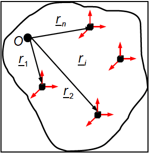
Figure description:
- Figure 527.2A-1: Diagram of a rigid body equipped with tri-axial linear accelerometers.
- Key Entities:
- Reference Point (: Origin point within the body.
- Accelerometers: Represented by black cubes with tri-axial red arrows indicating measurement axes.
- Position Vectors:
- : Vector from to the first accelerometer.
- : Vector from to the second accelerometer.
- : Vector from to an arbitrary -th accelerometer.
- : Vector from to the -th accelerometer.
- Context: Used for determining kinematics and 6-DOF (degree of freedom replication in laboratory testing.
In addressing the laboratory inputs required for 6-DOF replication, paragraph 6.1, references f and p also consider a body equipped with tri-axial linear accelerometers located as shown in Figure 527.2A-1. It is well known from classical mechanics that the acceleration measured by the transducer is given kinematically by
where represents the acceleration of a reference point in the body, and represent, respectively, the rigid body angular acceleration and angular velocity, the location of the transducer relative to the reference point, and represents the contributions due to non-rigid body effects (i.e., flexibility). Ignoring the flexibility effects (i.e., ), Equation 1 represents vector equations in three vector unknowns (i.e., , and ). In general, is unknown unless a transducer was selected a priori for that location. For notational convenience, matrix equivalent operations were used
Figure 527.2A-1: Body with accelerometers. Placements.
location. For notational convenience, matrix equivalent operations were used to rewrite Equation 1 as shown in Equation 2 where the flexibility effects have also been neglected.
In Equation (2), and are skew symmetric matrices representing the vector cross products, and represent the contributions of angular motion to the measured linear acceleration (i.e., the contributions of “tangential” and “centripetal” accelerations). Assuming that and are the angular acceleration and angular velocity coordinatized in the body fixed frame, then
, and
True motion replication in the laboratory using the measured accelerations (field data) to construct the drive point accelerations will require knowledge of a (three unknowns) and Q (nine unknowns), for a total of 12 unknowns. A closer examination of Q, however, reveals the matrix is comprised of only six unique unknowns (i.e., the == components of a and @). Thus, if a。, α, and @ can be determined from measured field data, theoretically, the motion in the field can be exactly (within the limits of the measurement devices) replicated in the laboratory. From paragraph 6.1, reference f, it was shown that in the most general case, nine parameters (ao,w,α) are required to reconstruct the motion and, thus, the minimum number of required transducer channels is nine. The analysis was also used to show that if specific restrictions are imposed on the motion (e.g., a₁ = 0), six properly placed accelerometers would be sufficient. Additionally, if consideration was given to the rigid body kinematic relationship between the do angular velocity @ and the angular acceleration α (i.e., α= ), then implementation in the frequency domain dt also reduces the number of required parameters from nine to six.
The two stated restrictions (i.e., a₁ = 0 or frequency domain implementation) that result in six transducers being sufficient, are consistent with the conditions found in the vibration testing environment. An assumption of a₁ = 0 does not necessarily provide sufficient information for exact motion reconstruction. In fact, it was shown that in the most general case, only a could be uniquely determined and, thus, additionally, the kinematic relationship between a and @ has to be exploited. Hence, the most influential of the two restrictions is the simplified relationship between angular velocity and angular acceleration in the frequency domain (i.e., α(s) = sw(s)). Note that this condition is
MIL-STD-810H
METHOD
527.2 ANNEX A
only valid for rigid bodies. Once flexibility is considered, this simplification no longer exists and, thus, the use of six transducers becomes questionable.
From an implementation perspective, while it has been shown that six properly located linear accelerometers are sufficient to use as a basis for 6-DOF motion replication, it is also obvious that near ideal conditions are required. Specifically, and as is generally the case for laboratory vibration tests, a 0 ≅ 0 in Equation 1 is a necessary requirement to ensure accurate replication of acceleration and velocity at unmonitored points on the test item. A more realistic concern is that, in practice, one is not necessarily working with a rigid body, and the fact that there will inevitably be a mechanical impedance mismatch between the field and laboratory conditions. Under such conditions, predictably there will be issues with the condition number of the system transfer function matrix H xy .
To address such issues, it is strongly recommended that an over-determined feedback scheme (number of control channels > number of mechanical DOF) consisting of properly placed linear accelerometers be employed. One such proven control configuration is selection of three non-collinear tri-axial clusters of linear accelerometers. This control configuration is very versatile in that any plane may be used, with the only critical factor being that the relative positions of the transducers remain non-collinear.
Downloaded from https://www.everyspec.com
MIL-STD-810H
METHOD
527.2 ANNEX A
(This page is intentionally blank.)
MIL-STD-810H METHOD 527.2 ANNEX B
METHOD 527.2, ANNEX B
SYSTEM IDENTIFICATION FOR LINEAR TIME-INVARIANT MDOF SYSTEMS
527.2 ANNEX B
for the SISO case, computation of both ˆH ( ) f and γ xy 2 ( ) f are simple division operations to be performed at each of the discrete spectral lines. The following paragraph takes a general MIMO view of the SISO scenario just discussed. In the following discussions, all estimates will be considered to be “smoothed” through the use of an appropriate number of measurements and the ^ symbol will be eliminated.
527.2 ANNEX B
| Gxxmm (f) = auto-spectrum of the input m |
| Gyynn (f) = auto-spectrum of the output n |
| Gxynn (f)=cross-spectrum between input m and output n |
527.2 ANNEX C
If possible, even though it may be band-limited, recommend an angular accelerometer or rate transducer be placed at the midpoint between the linear accelerometers being used to estimate the rotational DOF of interest. The addition of the angular accelerometer will provide a direct measure of ground truth for angular acceleration at a particular point on a structure.
527.2 ANNEX C
, represents the control channel number and the index, , represents the time segment number. For example, if the sample frequency is 1024 Hz, and the rms calculation is to be computed every 0.5 seconds ( samples), would represent samples , would represent the samples , and so on.
where, and
Step 3 Observing that the columns of the two matrices shown in Equation 3.2.2 represent the reference and laboratory test channels, g-rms values for a given time segment , it is possible to isolate the individual columns and develop a weighting strategy across all control channels for each time segment. Equation 3.2.3 illustrates a 2-norm computed for each column of the reference matrix . Note that post multiplication by indexing vector provides a method of isolating the column of interest.
Step 4 Equation 3.2.4 demonstrates computation of a weighting factor for each entry in the reference matrix , based on a column normalization to the corresponding 2-norm computed in Equation 3.2.3. This weighting factor may be considered in addressing rms-error between the reference and laboratory data.
(3.2.4)
Step 5 The relative error between the reference signals and signals measured during laboratory testing can be computed on a log scale per Equation 3.2.5.
MIL-STD-810H
METHOD 527.2 ANNEX C
RMS_ RMS_112 RMS_S RMS_11 RMS 12 RMS is RMS RMS RMS_25 (3.2.5) RMS_err=20 log10 RMS 21 RMS_22 RMS 2s JxS : RMS 1, RMS RMS RMS_л RMS_J2 RMS JS
Step 6 The RMS _err matrix can be normalized by the weighting parameter defined in Matrix Wt as illustrated in Equation 3.2.6.
(RMS_err₁₁)(W) (RMS_err₁₂) (W₁₁₂) (RMS_erris)(Wts) RMS Nerr= (RMS_err₂)(W) (RMS _err₂)(Wt) (RMS_err₂s)(Wt2s) (3.2.6) JxS ⠀ (RMS_err,) (Wt) (RMS_err√2) (Wt 12) (RMS_errs) (Wts),
Step 7
A Global-rms error may now be established for each time segment as illustrated in Equation 3.2.7.
Glob_rms err= Σ(RMS_Nerr)U₁,...) ,Σ (RMS_Nerr)\Us (3.2.7) 1xS j=1 j=1
The rms error produced in Step 7 above provides a global perspective to rms error between the reference and laboratory data in which each control location is included and weighted in terms of the energy within each time segment, s.
527.2 ANNEX C
BS the f index, f=1,F, where F = , represents each spectral line of the ASD estimate. For 2 example, if Fs = 1024 and the block-size (BS) used in the estimate of the ASD is set to BS = 512 Fs , F = 256 and the frequency resolution would be Af = =2Hz. In computing the ASD BS estimates, the time segment, s, may be either the entire range n = 1...N, or some subset thereof.
asdi asd IF asd_ asd F ASD_r(f)= ASD_1 = B (3.3.2) JxF asd_rл asd JF JxF asd _1л asd _1JF
Step 3 Observing that the columns of the two matrices shown in Equation 3.3.2 represent the reference and G² laboratory test channels values for a given spectral line as estimated over time segment, s, the Hz individual columns can be isolated and a weighting strategy developed across all control channels for each spectral line. Equation 3.3.3 illustrates a 2-norm computed for each column of the reference matrix ASD r. Post multiplication by indexing vector, U, provides a method of isolating an individual column of interest.
nc_asd_r = (( ASD _r; ) U₁||2,||(ASD _r¸ ) U2||2,···,||( ASD _r; )UF ||2|) 1xF
0 0 (3.3.3) where, U₁ = ... ,UF = Exl Exl
0
Step 4 Equation 3.3.4 demonstrates computation of a weighting factor for each entry in the reference matrix based on a column normalization to the corresponding 2-norm computed in Equation 3.3.3.
This weighting factor may be considered in addressing error between the reference and
laboratory data.
(ASD_1)² (ASD_112)² (ASD_F)² (nc_asd_r)² (nc_asd_r₂)² (nc_asd_r)² (ASD_1)² (ASD_122)² (ASD_2F)² Wt= (nc_asd_) (nc_asd_r₁₂)² JxF (nc_asd_r)² B (3.3.4) (ASD_)² (ASD_112)² (ASD_JF)² (nc_asd_r;)² (nc_asd_r₁₂)² (nc_asd_r)²
Step 5 The relative error between the reference signals and signals measured during laboratory testing can be computed on a log scale per Equation 3.3.5.
MIL-STD-810H
METHOD 527.2 ANNEX C
ASD ASD 1, ASD_F ASD_11 ASD 12 ASD_F ASD ASD ASD F ASD err =10log10 ASD_121 ASD_122 ASD_V2F (3.3.5) JxF B
ASD 1, ASD ASD ASD_л ASD_J2 ASD JF
Step 6 The matrix can be normalized by the weighting parameter defined in Matrix as illustrated in Equation 3.3.6.
((ASD_err₁₁) (Wt₁) (ASD_err₁₂)(Wt12) ... (ASD_err)(Wt₁F)` ASD Nerr= JxF (ASD_err)(W) (ASD_err₂2) (W22) B (ASD _err2F)(Wt2F) (3.3.6) ((ASD_err) (Wtɲ) (ASD_err₁₂) (Wt12) (ASD_err JF)(WtJF))
Step 7 A Global ASD error may now be established for each time segment, s , as illustrated in Equation 3.3.7.
The ASD error spectrum produced in Step 7 above provides a global perspective to ASD error between the reference and laboratory data in which each control location is included, and weighted in terms of the energy at each spectral line.
527.2 ANNEX D
composite set of reference spectra for a MEMA test. The difficulty lies primarily in the inability to characterize the CSD terms across an ensemble of measurements. This issue is discussed in further detail in Annex E.
527.2 ANNEX D
A control measurement point would typically be on a structural member and describe the overall vibration characteristics of the item. A monitoring measurement point would describe local vibration characteristics that are relevant for a specific component. Paragraph 6.1, reference j, provides information on extremes of excitation.
527.2 ANNEX E
(i.e., X-, Y-, Z-translations and roll, pitch, yaw rotations). In some cases, additional DOFs can be excited due to deformations of the test article and/or testing an item with articulating components.
527.2 ANNEX E
- c. Minor errors in the matching of shakers can be corrected by the control algorithm, but major mismatches could be problematic. The time domain drive signals (represented by {s}), are sent to the shakers completing the control loop.
- d. If is not available, then and . If is not available, then and . If , the number of control variables and the number of drive variables are the same. This is referred to as square control. Square control is the most common control method. If the system is over-actuated and least squares approach using a pseudo inverse (pinv) is typically used to determine the drive signals. If the system is under-actuated and exact control of the control SDM is often not possible. In such cases, some kind of average control is usually implemented. Often when some combination of the transformation matrices are often used to force square control, .
- e. The entire mechanical system can be characterized by a matrix of frequency response functions [H]. For the typical case, these frequency response functions will have units of g/V (acceleration in gravitational units/volts of drive). For the typical case, the control signals are characterized by a SDM. The diagonal elements are the autospectral density (ASD or PSD) of the control signals. The off diagonal elements are the cross spectral densities (CSD) between pairs of control signals. The input to the system is characterized by the SDM of the voltage drive signals. The fundamental relationship between the drives and the control signals is given by:
C = HDH'
- f. The complex conjugate transpose is denoted by ( )'. All of the matrices in the equation are complex functions of frequency. The spectral density matrix is Hermitian, i.e. Dij = Dji * where Dj¡ * is the complex ji conjugate of Dj;, and Dj; is an element from a spectral density matrix. Note that this requirement demands ji' ji that the diagonal elements are real. Note that C and D are square matrices; they have the same number of rows and columns. C and D are the same size only if H is square, i.e. the same number of inputs and outputs. To be physically realizable, the SDM must also be positive semi-definite. This requirement will be discussed in paragraph 4.5.2.
- g. The drive spectral density matrix is converted into the drive time histories using the method of time domain randomization4. The spectral density matrix is typically estimated using Welch’s method7.
527.2 ANNEX E
527.2 ANNEX E
control variables. Often these control variables are descriptions of rigid body modes. The acceleration transformation is usually performed in the time domain as:
{c} = {a}
527.2 ANNEX E
- (1) Case 1: Configurations in which the number of motion degrees-of-freedom or control signals, N and the number of output control variables, Na are the same is referred to as "square" control. If the d number of output control variables, Nd and the number of shakers, N, is the same, the transformation matrix, Ts will simply be the Identity matrix.
- (2) Case 2: Configurations in which the number of shakers N¸ exceeds the number of output control variables Nd, the excitation system is said to be over-determined or over-actuated. In such cases, some of the drives will be linear combinations of other drives. Furthermore, if Ts is a constant which is employed in the time domain, the individual actuators must be matched (e.g. matched frequency response functions (FRFs)).
- (3) Case 3: Configurations in which the number of shakers, N¸ is less than the number of control signals, Ne, the excitation system is said to be under-determined or under-actuated. In such cases, exact control of the SDM is not possible.
- b. In theory, Ts could be implemented before or after the transformation into the time domain. One advantage of placing the transformation in the frequency domain section of the control algorithm is that the matrix could then be made a function of frequency. Having the transformation matrix, Ts, a constant assumes the shakers are matched and the desired transformation can be deduced.
527.2 ANNEX E
time histories will be referenced to a single point on the structure referred to as the “origin” as discussed in paragraph4.4.1.
- b. A SDM for each test configuration identified in the mission scenario should be computed. In addressing the VSD techniques for reducing an ensemble of data, in this case an ensemble of SDM's, the analyst will be required to deal with the ASD terms (the diagonal terms of the SDM) and CSD terms (the off-diagonal terms of the SDM).
527.2 ANNEX E
interpreted as the auto-spectral densities of independent random noise sources. The maximum number of independent noise sources is N. If some of the elements in I are zero, the problem can still be solved by making the corresponding rows and columns of L zero. This is the positive semi-definite case. This case corresponds to the case where there exists less than N independent sources. Some of the N sources are linear combinations of other sources. This case will be very difficult for the control system. In general one may make some of the sources small but not zero. Part of this document will discuss the generation of a desired control SDM to make the control problem achievable and hopefully relatively easy for the control system to implement.
- c. In general the control problem is an inverse problem. The desired control SDM (the output of the system under test) is known, and the drive (input to the system under test) SDM must be computed. There is a potential point of confusion here. The control system manufacturers treat the drive SDM as the output of the control system, which is the input to the shaker system. Similarly, the control system input is the output of the shaker system. Paragraphs 4.4.1 and 4.4.2 provide nomenclature employed for input and output transformations as they are applied within this document.
- d. Inverse problems can be very difficult as multiplication by a matrix inverse is required. If the matrix is ill-conditioned, the result will be similar to dividing by zero for the scalar case.
For the case in which the number of inputs and outputs are the same; H is a square matrix of FRF’s. The solution is to invert H. The solution for the drive matrix is then given by:
Z=H-¹ D = ZRZ'
This of course assumes H is well conditioned and the inverse exists. Part of this document will discuss issues to help the process of achieving a well conditioned H matrix.
The H matrix is typically estimated from:
-1
The inverse of Dˆ must exist. This implies that Dˆ must be positive definite. The initial estimate of H is determined by exciting the system with a set of independent white inputs in a pretest environment. If H is to be corrected during the test, Dˆ must be positive definite during the test or special provisions must be used to avoid the inversion of Dˆ at frequencies where Dˆ is not positive definite. This is one of the reasons the reference R rarely has any of the coherences equal to unity.
527.2 ANNEX E
= severity (root mean square ((rms)) at test condition = severity (rms) at in-service condition (The ratio is commonly known as the exaggeration factor.)
a value based on (but not equal to) the slope of the S-N curve for the appropriate material where S represents the stress amplitude and N represents the mean number of constant amplitude load applications expected to cause failure. For the MDOF VSD work at hand, the default of was selected per reference number 1 .
- b. It is recommended that the final vibration specification ASD terms are no greater than 3 decibel (dB) higher than maximum values measured in the field. Miner-Palmgren will be employed to the ASD portion of the SDM in the same manner as one would employ for a traditional 1-DOF scenario. Details such as maintain common test durations between mechanical DOFs are addressed in Paragraph 6.
527.2 ANNEX E
Y = diag(Sy). The relationship between the autospectra, as shown in Appendix D proof 1, is given by:
Y = HX where:
where: * indicates an element by element multiplication. .
The solution is given by:
- b. In some cases the result will include negative elements in . This is not physically possible. It indicates that the desired ASD's cannot be achieved with independent drives. In this case the negative values are set to zero, and the output SDM is recomputed from using the modified input spectral density matrix (the negative values set to zero). The resulting control point acceleration autospectra, will not be at the desired levels. To correct this problem, the control point acceleration autospectra are rescaled to the desired levels, keeping the phase and ordinary coherence the same. This is accomplished by pre and post multiplying the SDM by a diagonal matrix whose elements are the square root of the ratio of the desired ASD to the computed ASD:
where Ss is a diagonal matrix and:
Note: Setting , provides an efficient way to compute the normalized SDM where the diagonals are one and the magnitude of the off diagonals squared are the ordinary coherence and the phase of the off diagonal elements is the phase of the cross spectra.
The drive SDM can then be computed as:
where , the Moore-Penrose pseudo inverse. If H is square and full rank, the solution typically ends here. If H is not square or not full ranked:
Synew=HS, Xnew H'
The may not yield the desired ASD's. In this case, an iterative approach will often improve the result.
527.2 ANNEX E
data were taken may not be identical to the test vehicle. Fifth, the boundary conditions in the field may be different from the boundary conditions in the laboratory.
- b. Small changes in the modal frequencies caused by any of the above factors can change the phase at any frequency near a mode by a large amount. All these factors make the specification of the cross spectra difficult. An option is to ignore the cross spectra and set them all to zero. This has the theoretical advantage of providing an excitation that in some sense covers the control variable response space.
- c. The drive signals can readily be computed yielding uncorrelated motion (in this case the SDM of the uncorrelated reference spectra Y is diagonal) from:
Sxo = ZS YoZ' ΧΟ
This approach is currently available in commercial control systems. You simply specify the reference SDM as a diagonal matrix with the cross spectra (or equivalently the coherences) zero or near zero. This is typically a conservative approach.
- d. In contrast to the independent drive discussion in paragraph 4.5.5.1, the danger with the independent reference concept is that this specification of control variables may be overly conservative near frequencies dominated by a single mode. An important clue that the result may be overly conservative is the trace of the drive voltages. This trace should be monitored and if overly large in some band of frequencies, limits can be negotiated and implemented.
527.2 ANNEX E
527.2 ANNEX E
address this situation in varying degrees, it may still be necessary to address this issue through test operator intervention via techniques such as those identified in paragraphs 4.5.4 and 4.5.5.
527.2 ANNEX E
Identify position vectors and row selection vectors as defined in paragraph 4.4.1.1, corresponding to the field measurements.
Identify the mission scenario.
Identify the frequency bandwidth of interest.
Identify the sampling frequency of the field measurements.
- Step 2 Transform the field measurements into motion DOF's per equation (4.3) for each "Run" identified in the mission scenario.
- Step 3 Compute the SDM for each run identified in Step 2. The dimension of the resulting SDM’s will be [6x6xd], where d is the number of spectral lines being considered to addresses the frequency bandwidth of interest.
Since the SDM is computed from measured field data, it should be positive definite; however, a check should be performed to verify that each individual SDM is positive definite. This serves as an excellent data quality check.
Refer to the guidance in Step 7 if minor corrections are required to force an individual SDM to be positive definite.
Step 4 Convert the CSD terms (the off-diagonal terms of the SDM) into a normalized form in which the magnitude squared of the cross terms correlates to the ordinary coherence while leaving the phase unchanged.
This is accomplished by normalizing (dividing) the CSD terms by .
While it is not absolutely necessary to conduct this step, it is often easier to understand the physical meaning of the CSD terms when viewed in terms of phase and coherence.
Step 5 Either organize all of the SDM’s for the Runs of interest into a logical structure or merge them into one file of known matrix structure such as [SDM_Run1,SDM_Run2….SDM_RunN] to optimize the conduct of basic statistics.
Step 6 Compute a weighted average SDM of the N SDM's of Step 5.
It is critical that the weighted average be performed on the true complex CSD terms (not the normalized SDM).
The weighting factor on the average will be directly correlated to the mission scenario times identified in Step 1. If the individual Runs are positive definite, the resulting average should also be positive definite. However, numerical issues may yield non-positive definite results. To minimize numerical issues, average only the lower triangular portion of the SDM and fill in the upper triangular portion of the SDM by taking advantage of the Hermitian structure of the matrix [16].
Any type of enveloping operation should be avoided as it is highly likely to yield a non-positive definite result.
Step 7 As SDM data are manipulated through activities such as averaging, it is advisable to verify the results remain positive definite. As discussed above, occasional numerical issues may be of concern in some instances. If required, force the SDM computed in Step 6 to be positive definite.
This is done by systematically reducing the magnitude of the cross spectral density terms until the Cholesky decomposition is possible at each depth (spectral line) of the SDM. (If required, this process may be somewhat conservative in its reduction of the coherence between DOFs in that the systematic reduction of cross term magnitudes is applied to each cross term equally).
Step 8 Scale the diagonal terms of the autospectra (the diagonal terms of the SDM) resulting from Step 7 to the maximum rms level of each of the N SDM's in Step 5 on an individual DOF basis using Miner-Palmgren.
MIL-STD-810H METHOD
527.2 ANNEX E
Observe that a new total test time will be computed for each DOF and that it is highly probably that the resulting test times for each DOF will not be the same.
Since the magnitude of the autospectra are being increased while not modifying the cross-spectral density terms, the resulting scaled SDM should still be positive definite. However, as discussed in Step 7, it is highly recommended that anytime a SDM is manipulated, it should be verified that the resulting SDM remains positive definite.
Step 9 Review the test time associated with each DOF resulting from Step 8 and select a reasonable test time to which the entire SDM may be referenced to. In this step, avoid scaling the dominant DOF by more than the maximum envelope of measured values for that DOF.
Just as in the case of a 1-DOF VSD development, one should consider the general guidance to keep the final test amplitudes resulting from time compression to be no more than 3 dB above the maximum measured field data. Once a test time is selected, reapply Miner-Palmgren as required per DOF. Again make sure the resulting SDM is positive definite and modify as required per Step 7.
Step 10 Scale the results from Step 9 up by up to 3 dB, while not exceeding 3dB above the envelope of measured values per DOF, to account for uncontrolled variables such as fleet variations and scenario conditions not considered in the mission scenario. There are often practical limitations in maintaining all DOF’s within 3 dB of the envelope of measured values from their respective DOF. In such cases, attempt to associate the maximum compression with the lowest level DOF or a DOF known to be mechanically robust. The resulting SDM and the test time association per Step 9 define the final specification.
This is accomplished by pre and post multiplying the SDM by the square root of the ratio of the desired scaling factor as:
(e.g. to scale the SDM ASD terms by 3 dB while keeping the phase and ordinary coherence the same, the diagonal terms of would be defined as ).
[In the event the user has documented evidence that the mission scenario is of sufficient fidelity to minimize uncontrolled variables, the default scale factor of 3 dB in this step may be reduced].
527.2 ANNEX E
of the ASD terms will not be the same. In addition, the spectral shape of the ASD terms will generally have been slightly modified.
- Step 7 Rescale the ASD terms of the SDM resulting from Step 6 to match the rms levels of those in Method 1 Step 6.
Convert the CSD terms (the off-diagonal terms of the SDM) into a normalized form in which the magnitude squared of the cross terms correlates to the ordinary coherence while leaving the phase unchanged. (Again, while it is not absolutely necessary to conduct this step, it is often easier to understand the physical meaning of the CSD terms when viewed in terms of phase and coherence).
Observe that Method II involves the averaging of matrix square roots. The resulting SDM phase and coherence are expected to be very similar to those of the averaged field data produced in Method I. The ASD terms spectral shapes are expected to be slightly different (i.e. < 3 dB per spectral line for SDM's of similar statistical variance). The actual differences depend to a great deal on the statistical variation of the component square roots. If the statistical variation is significant, one may consider developing multiple references by grouping runs with similar spectral shapes or by reverting to Method I.
Step 8-10 Correlate directly to Method I Outline.
527.2 ANNEX E
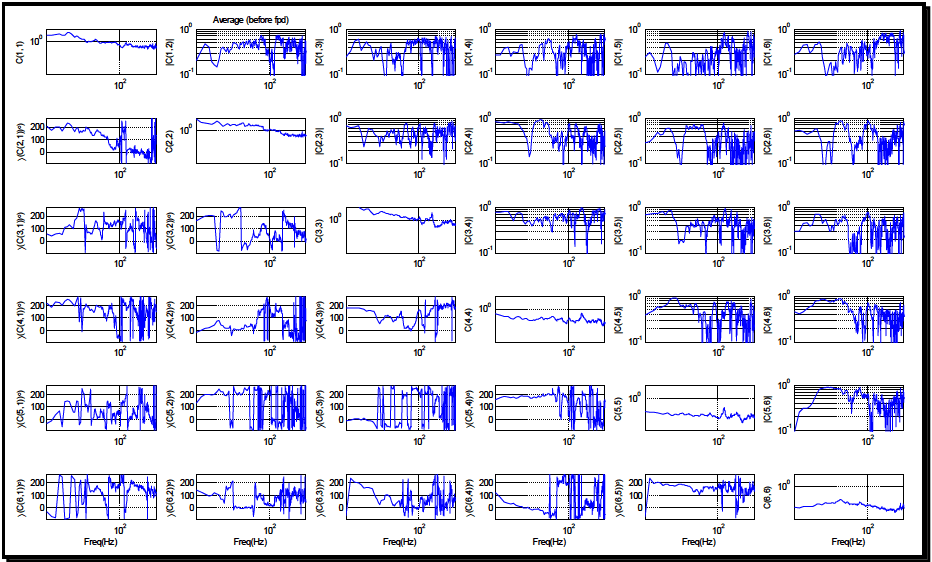
Figure description:
Matrix of Average Frequency Responses (before fpd
Average (before fpd
| Freq(Hz) | C(1,1) | |C(1,2)| | |C(1,3)| | |C(1,4)| | |C(1,5)| | |C(1,6)| | ∠C(2,1°) | C(2,2) | |C(2,3)| | |C(2,4)| | |C(2,5)| | |C(2,6)| | ∠C(3,1°) | ∠C(3,2°) | C(3,3) | |C(3,4)| | |C(3,5)| | |C(3,6)| | ∠C(4,1°) | ∠C(4,2°) | ∠C(4,3°) | C(4,4) | |C(4,5)| | |C(4,6)| | ∠C(5,1°) | ∠C(5,2°) | ∠C(5,3°) | ∠C(5,4°) | C(5,5) | |C(5,6)| | ∠C(6,1°) | ∠C(6,2°) | ∠C(6,3°) | ∠C(6,4°) | ∠C(6,5°) | C(6,6) | |---|---|---|---|---|---|---|---|---|---|---|---|---|---|---|---|---|---|---|---|---|---|---|---|---|---|---|---|---|---|---|---|---|---|---|---|---|---|---| | 20 | 1.5 | 0.3 | 0.4 | 0.3 | 0.2 | 0.4 | 180 | 3.0 | 0.4 | 0.6 | 0.3 | 0.5 | 50 | 0 | 1.8 | 0.5 | 0.6 | 0.5 | 230 | 0 | 200 | 0.8 | 0.2 | 0.3 | 0 | 180 | 0 | 150 | 0.5 | 0.1 | 0 | 100 | 210 | 100 | 200 | 0.4 | | 40 | 2.0 | 0.5 | 0.6 | 0.4 | 0.4 | 0.5 | 170 | 2.5 | 0.5 | 0.8 | 0.5 | 0.4 | 60 | 5 | 2.5 | 0.8 | 0.7 | 0.4 | 240 | 20 | 220 | 0.7 | 0.4 | 0.2 | 50 | 200 | 10 | 160 | 0.45 | 0.8 | 220 | 90 | 190 | 60 | 210 | 0.5 | | 60 | 1.2 | 0.4 | 0.5 | 0.3 | 0.2 | 0.4 | 180 | 2.2 | 0.4 | 0.3 | 0.3 | 0.2 | 180 | 200 | 1.8 | 0.5 | 0.4 | 0.2 | 200 | 80 | 150 | 0.6 | 0.5 | 0.1 | 150 | 220 | 20 | 170 | 0.4 | 0.6 | 100 | 110 | 100 | 30 | 190 | 0.6 | | 80 | 1.0 | 0.4 | 0.4 | 0.2 | 0.3 | 0.3 | 150 | 2.0 | 0.3 | 0.4 | 0.4 | 0.3 | 150 | 150 | 1.5 | 0.4 | 0.3 | 0.1 | 150 | 60 | 100 | 0.5 | 0.4 | 0.3 | 120 | 210 | 150 | 160 | 0.4 | 0.7 | 50 | 60 | 60 | 20 | 150 | 0.7 | | 100 | 1.0 | 0.3 | 0.3 | 0.3 | 0.3 | 0.3 | 100 | 1.8 | 0.3 | 0.4 | 0.4 | 0.3 | 100 | 20 | 1.0 | 0.5 | 0.5 | 0.2 | 100 | 50 | 50 | 0.5 | 0.3 | 0.4 | 100 | 180 | 100 | 150 | 0.4 | 0.5 | 100 | 50 | 50 | 20 | 100 | 0.6 | | 150 | 0.8 | 0.6 | 0.5 | 0.6 | 0.5 | 0.6 | 50 | 1.2 | 0.6 | 0.7 | 0.6 | 0.5 | 80 | 80 | 1.1 | 0.7 | 0.6 | 0.7 | 50 | 100 | 80 | 0.6 | 0.7 | 0.6 | 80 | 100 | 80 | 100 | 0.45 | 0.8 | 150 | 80 | 100 | 50 | 80 | 0.5 | | 200 | 0.7 | 0.4 | 0.4 | 0.4 | 0.4 | 0.4 | 150 | 1.0 | 0.4 | 0.4 | 0.4 | 0.3 | 160 | 150 | 1.0 | 0.4 | 0.4 | 0.5 | 180 | 210 | 180 | 0.7 | 0.4 | 0.4 | 180 | 150 | 150 | 180 | 0.5 | 0.4 | 210 | 120 | 180 | 120 | 160 | 0.4 | | 250 | 0.6 | 0.5 | 0.6 | 0.5 | 0.6 | 0.5 | 10 | 0.9 | 0.7 | 0.6 | 0.5 | 0.6 | 50 | 50 | 0.8 | 0.6 | 0.5 | 0.4 | 120 | 80 | 120 | 0.6 | 0.5 | 0.4 | 50 | 80 | 20 | 80 | 0.45 | 0.6 | 80 | 40 | 60 | 40 | 100 | 0.3 | | 300 | 0.5 | 0.3 | 0.3 | 0.2 | 0.3 | 0.2 | 0 | 0.8 | 0.2 | 0.2 | 0.2 | 0.3 | 100 | 40 | 0.9 | 0.3 | 0.3 | 0.3 | 100 | 150 | 100 | 0.5 | 0.2 | 0.2 | 100 | 100 | 100 | 100 | 0.4 | 0.2 | 100 | 100 | 100 | 50 | 100 | 0.5 |
Notes: The 6x6 grid represents a matrix of frequency responses. Diagonal elements and upper-triangle elements are magnitude responses (log scale on y-axis. Lower-triangle elements are phase responses in degrees (linear scale on y-axis, 0 to 200. All plots share a common logarithmic x-axis for frequency in Hz, ranging from approximately 20 Hz to 300 Hz.)))))
Figure 5. Normalized weighted average SDM.
- (9) Per Step 9, the new test times associated with each ASD were also documented. As expected, the new times associated with each DOF were no longer the same. Since the VSD effort is designed to yield a simultaneous 6-DOF reference, it will be necessary to choose a common test time and rescale all ASD entries to the selected test duration. For the example at hand, a test duration of 15 minutes was selected. As is always the case with selection of compressed test durations, one should adhere to the guidance of not exaggerating the ASD power levels by more than 2:1. Of course when dealing with 6 ASD terms, this is not always possible. In such cases, the analyst should avoid increasing the dominant DOFS or DOFS with known structural shortcomings by more than 3 dB above maximum measured ASD levels.
- (10) The terms comprising the SDM were based on average ASD and CSD estimates, which is in contrast to the guidance provided in reference number 3, in which the ASD levels carried through the calculations of a 1-DOF VSD were actually based on an ASD computed as the sum of a Mean ASD and standard deviation computed on a per spectral line basis. Working directly with the mean ASD levels is intended to avoid excessive conservatism in the VSD process. Conservatism intended to address uncontrolled variables such as fleet variations and conditions not considered in the mission scenario are addressed by a single scalar (+3 dB in this example) in Step 10. Clearly the analyst has the ability to modify the final conservatism level based on knowledge of the specific VSD effort.
The final reference SDM produced by Method I is shown in Figure 6. Observe that the phase and coherence terms are essentially unchanged from that of the average SDM of Figure 5.
MIL-STD-810H METHOD 527.2 ANNEX E
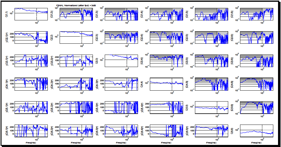
Figure description:
FINAL Normalized (after fpd +3dB”, “additional_notes”: “The figure displays a 6x6 matrix of plots representing the frequency response of a normalized system. Diagonal plots C(i,i and top-right off-diagonal plots |C(i,j| show magnitudes on a logarithmic y-axis (ranging from approximately 0.1 to 10. Bottom-left off-diagonal plots ∠(C(i,j° show phase responses on a linear y-axis from 0 to 200 degrees. Frequency is shown on a logarithmic x-axis centered around 100 Hz.
Normalized Matrix Components C(i,j
Annotations
- 100 Hz Center Reference (vertical_line - position: x = 100)
- Unity Magnitude (Log Scale (horizontal_line - position: y = 10^0 (1.0 on diagonal and top-right plots)))
- Phase Reference Lines (horizontal_line - position: y = 0, 100, 200 on bottom-left phase plots)
| Freq(Hz) | C(1,1) | |C(1,2)| | |C(1,3)| | |C(1,4)| | |C(1,5)| | |C(1,6)| | ∠(C(2,1°)) | C(2,2) | |C(2,3)| | |C(2,4)| | |C(2,5)| | |C(2,6)| | ∠(C(3,1°)) | ∠(C(3,2°)) | C(3,3) | |C(3,4)| | |C(3,5)| | |C(3,6)| | ∠(C(4,1°)) | ∠(C(4,2°)) | ∠(C(4,3°)) | C(4,4) | |C(4,5)| | |C(4,6)| | ∠(C(5,1°)) | ∠(C(5,2°)) | ∠(C(5,3°)) | ∠(C(5,4°)) | C(5,5) | |C(5,6)| | ∠(C(6,1°)) | ∠(C(6,2°)) | ∠(C(6,3°)) | ∠(C(6,4°)) | ∠(C(6,5°)) | C(6,6) | |---|---|---|---|---|---|---|---|---|---|---|---|---|---|---|---|---|---|---|---|---|---|---|---|---|---|---|---|---|---|---|---|---|---|---|---|---|---|---|---|---|---|---|---|---|---|---| | 40 | 5.0 | 0.3 | 0.4 | 0.3 | 0.3 | 0.4 | 180 | 6.0 | 0.5 | 0.4 | 0.4 | 0.5 | 50 | 180 | 6.0 | 0.5 | 0.3 | 0.4 | 120 | 50 | 100 | 1.2 | 0.5 | 0.4 | 80 | 180 | 10 | 150 | 0.8 | 0.4 | 120 | 150 | 150 | 100 | 180 | 0.4 | | 100 | 2.0 | 0.5 | 0.3 | 0.5 | 0.4 | 0.4 | 100 | 3.0 | 0.3 | 0.4 | 0.3 | 0.4 | 100 | 150 | 2.0 | 0.4 | 0.3 | 0.3 | 100 | 100 | 100 | 1.0 | 0.4 | 0.4 | 100 | 100 | 100 | 100 | 0.8 | 0.4 | 100 | 100 | 100 | 100 | 100 | 0.6 | | 250 | 2.5 | 0.4 | 0.5 | 0.4 | 0.6 | 0.5 | 20 | 2.0 | 0.4 | 0.3 | 0.4 | 0.5 | 150 | 50 | 4.0 | 0.3 | 0.4 | 0.4 | 50 | 120 | 50 | 1.0 | 0.5 | 0.5 | 150 | 80 | 150 | 50 | 0.6 | 0.3 | 50 | 150 | 80 | 150 | 40 | 0.4 |
Figure 6. Method I normalized reference SDM.
- c. Method II Example. The first four steps of Method II correlate directly to that of Method I. The major deviation in Method II is that all averaging will be computed in the Cholesky domain. In Step 5, Cholesky decompositions are carried out on the individual SDM's associated with each Run in the mission scenario. Since each individual Run was based on a measured physical event, the individual SDMs were positive definite as expected, thereby making the Cholesky decomposition possible. In the event that a given Run had failed the Cholesky decomposition and all measurement locations and relative polarities were verified; investigate the spectral lines at which the decomposition fails. If the decomposition is failing at only a few spectral lines, it may be possible to salvage the measurement employing the CSD magnitude reduction techniques proposed in Method I. The Cholesky domain data were then organized into a convenient structure for statistical analysis. As in Method I, Matlab was used to compute the weighted averages and the Cholesky domain data were organized as: CHOL_all=[CHOL_Run1, CHOL_Run2 ,CHOL_RunN]. In Step 6, a weighted average in terms of the time per road condition as defined in Table 1 was computed over the lower triangular matrix of the eight Cholesky decompositions of Step 5. The weighted average was then converted back into the SDM domain. As expected, the coherence characteristics of the resulting SDM were comparable with that of Figure 5 and the rms levels of the ASD terms required rescaling per Step 7. Steps 8-10 were carried out directly as stated in the Method I outline.
- d. The reference SDM resulting from Method II (Figure 7) yielded similar phase and coherence characteristics to that of the reference SDM resulting from Method I (Figure 6). Note that the Method I example took advantage of averaging only the lower triangular CSD terms, avoiding potential numerical issues, thereby not requiring the SDM to be forced positive definite in a manner that would result in lowering the coherence in a more conservative manner than required.
- e. ASD Comparisons. Next, the minor spectral shape deviations between the ASD resulting from the two VSD methods discussed will be illustrated. Figures 8 and 9 show the ASD references for the Z axis (vertical) and rotation about Z axis (RZ) respectively, as produced from both VSD methods. The ASD references are superimposed with the raw (unexaggerated) reference data from which the specifications were created. Observe that the ASD shapes envelope the field data without excessive conservatism.
MIL-STD-810H METHOD 527.2 ANNEX E
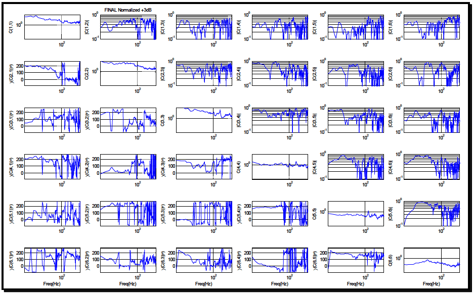
Figure description:
Normalized Cross-Spectral Estimates Matrix Cross-spectral magnitude and phase relationship between 6 signals
FINAL Normalized +3dB Matrix
Annotations
- 100 Hz Frequency Marker (vertical_line - position: x = 100)
- Unity Reference (horizontal_line - position: y = 1.0 (log for magnitude plots))
| Freq(Hz) | C(1,1) | |C(1,2)| | |C(1,3)| | |C(1,4)| | |C(1,5)| | |C(1,6)| | ∠(C(2,1°)) | C(2,2) | |C(2,3)| | |C(2,4)| | |C(2,5)| | |C(2,6)| | ∠(C(3,1°)) | ∠(C(3,2°)) | C(3,3) | |C(3,4)| | |C(3,5)| | |C(3,6)| | ∠(C(4,1°)) | ∠(C(4,2°)) | ∠(C(4,3°)) | C(4,4) | |C(4,5)| | |C(4,6)| | ∠(C(5,1°)) | ∠(C(5,2°)) | ∠(C(5,3°)) | ∠(C(5,4°)) | C(5,5) | |C(5,6)| | ∠(C(6,1°)) | ∠(C(6,2°)) | ∠(C(6,3°)) | ∠(C(6,4°)) | ∠(C(6,5°)) | C(6,6) | |---|---|---|---|---|---|---|---|---|---|---|---|---|---|---|---|---|---|---|---|---|---|---|---|---|---|---|---|---|---|---|---|---|---|---|---|---| | 30 | 4.12 | 0.52 | 0.38 | 0.28 | 0.31 | 0.44 | 185 | 5.10 | 0.32 | 0.41 | 0.29 | 0.33 | 55 | 182 | 4.80 | 0.28 | 0.37 | 0.31 | 195 | 12 | 178 | 1.15 | 0.33 | 0.42 | 15 | 148 | 8 | 185 | 0.62 | 0.18 | 12 | 195 | 205 | 45 | 198 | 0.52 | | 50 | 2.45 | 0.48 | 0.55 | 0.35 | 0.42 | 0.33 | 165 | 4.20 | 0.45 | 0.32 | 0.38 | 0.25 | 75 | 195 | 3.90 | 0.35 | 0.32 | 0.45 | 210 | 18 | 165 | 0.98 | 0.42 | 0.51 | 35 | 165 | 22 | 175 | 0.55 | 0.32 | 25 | 215 | 145 | 38 | 195 | 0.61 | | 100 | 1.48 | 0.65 | 0.45 | 0.52 | 0.33 | 0.58 | 15 | 1.25 | 0.52 | 0.41 | 0.33 | 0.45 | 155 | 18 | 1.45 | 0.58 | 0.38 | 0.42 | 12 | 15 | 12 | 0.85 | 0.12 | 0.25 | 155 | 15 | 175 | 18 | 0.58 | 0.44 | 18 | 12 | 15 | 22 | 15 | 0.48 | | 150 | 1.18 | 0.45 | 0.58 | 0.32 | 0.45 | 0.38 | 8 | 1.35 | 0.38 | 0.48 | 0.35 | 0.32 | 95 | 105 | 2.40 | 0.32 | 0.35 | 0.48 | 175 | 115 | 155 | 0.92 | 0.52 | 0.15 | 95 | 125 | 95 | 155 | 0.52 | 0.28 | 145 | 105 | 105 | 155 | 125 | 0.42 | | 300 | 1.55 | 0.32 | 0.48 | 0.55 | 0.22 | 0.35 | 2 | 1.58 | 0.32 | 0.25 | 0.52 | 0.58 | 55 | 45 | 1.35 | 0.55 | 0.42 | 0.35 | 85 | 145 | 105 | 1.05 | 0.25 | 0.42 | 55 | 85 | 55 | 105 | 0.45 | 0.22 | 105 | 55 | 105 | 55 | 85 | 0.51 |
Notes: The 6x6 matrix displays Cross-Spectral Density estimates. Diagonal elements are autospectra C(i,i on log scales. Upper triangle elements represent cross-spectral magnitudes |C(i,j| on log scales. Lower triangle elements represent cross-spectral phase angles ∠(C(i,j° on linear scales ranging from 0 to 200 degrees. Frequency is displayed on a logarithmic axis.))))
Figure 7. Method II reference SDM.
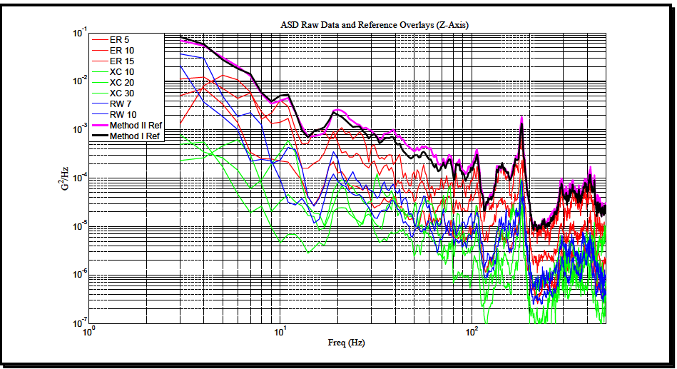
Figure description:
ASD Raw Data and Reference Overlays (Z-Axis
ASD Raw Data and Reference Overlays (Z-Axis
Legend
- ER 5 — color: red; symbol: thin solid line
- ER 10 — color: red; symbol: thin solid line
- ER 15 — color: red; symbol: thin solid line
- XC 10 — color: green; symbol: thin solid line
- XC 20 — color: green; symbol: thin solid line
- XC 30 — color: green; symbol: thin solid line
- RW 7 — color: blue; symbol: thin solid line
- RW 10 — color: blue; symbol: thin solid line
- Method II Ref — color: magenta; symbol: thick solid line
- Method I Ref — color: black; symbol: thick solid line
| Freq (Hz) | ER 5 | ER 10 | ER 15 | XC 10 | XC 20 | XC 30 | RW 7 | RW 10 | Method II Ref | Method I Ref |
|---|---|---|---|---|---|---|---|---|---|---|
| 3.0 | 0.0012 | 0.004 | 0.06 | 0.00022 | 0.00035 | 0.0008 | 0.02 | 0.04 | 0.08 | 0.08 |
| 5.0 | 0.008 | 0.011 | 0.032 | 0.0003 | 0.00004 | 0.0004 | 0.0022 | 0.03 | 0.05 | 0.05 |
| 8.0 | 0.0004 | 0.015 | 0.006 | 0.00002 | 0.00001 | 0.00015 | 0.002 | 0.0004 | 0.015 | 0.015 |
| 10.0 | 0.0003 | 0.0004 | 0.004 | 0.000006 | 0.000018 | 0.00008 | 0.00004 | 0.00015 | 0.004 | 0.004 |
| 15.0 | 0.0003 | 0.00025 | 0.0003 | 0.0000035 | 0.000004 | 0.00003 | 0.00002 | 0.00004 | 0.0008 | 0.0008 |
| 20.0 | 0.0011 | 0.0004 | 0.0009 | 0.000015 | 0.00003 | 0.0001 | 0.00012 | 0.0001 | 0.0025 | 0.0023 |
| 30.0 | 0.0008 | 0.00025 | 0.00035 | 0.000007 | 0.000008 | 0.00003 | 0.00003 | 0.00005 | 0.0011 | 0.001 |
| 50.0 | 0.00025 | 0.00005 | 0.00015 | 0.000004 | 0.000005 | 0.000015 | 0.00004 | 0.00002 | 0.0004 | 0.0003 |
| 80.0 | 0.0003 | 0.00015 | 0.00008 | 0.000003 | 0.000002 | 0.00001 | 0.000015 | 0.00001 | 0.0002 | 0.00018 |
| 100.0 | 0.00004 | 0.00008 | 0.00025 | 0.0000008 | 0.000001 | 0.000005 | 0.000004 | 0.000015 | 0.00025 | 0.00022 |
| 180.0 | 0.0002 | 0.0003 | 0.0004 | 0.00005 | 0.00006 | 0.0001 | 0.000035 | 0.00002 | 0.0018 | 0.0015 |
| 300.0 | 0.00005 | 0.00007 | 0.000035 | 0.000003 | 0.000006 | 0.000015 | 0.000008 | 0.000004 | 0.00008 | 0.00007 |
| 500.0 | 0.00003 | 0.000015 | 0.00002 | 0.0000015 | 0.000002 | 0.000004 | 0.0000015 | 0.0000011 | 0.00004 | 0.000035 |
Figure 8. ASD references for the Z axis.
MIL-STD-810H METHOD
527.2 ANNEX E
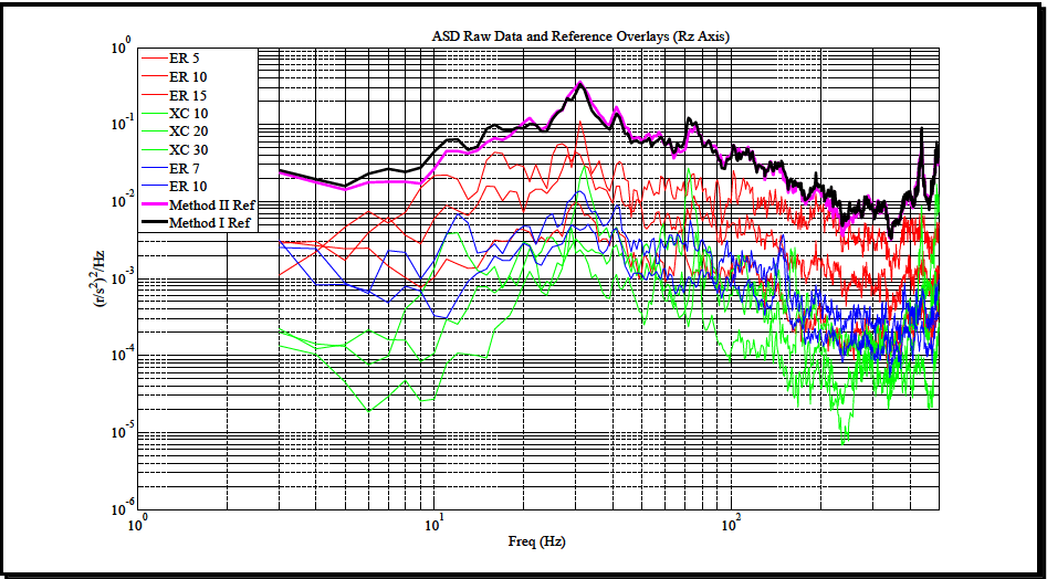
Figure description:
ASD Raw Data and Reference Overlays (Rz Axis
ASD Raw Data and Reference Overlays (Rz Axis
Legend
- ER 5 — color: red; symbol: thin solid line
- ER 10 — color: red; symbol: thin solid line
- ER 15 — color: red; symbol: thin solid line
- XC 10 — color: green; symbol: thin solid line
- XC 20 — color: green; symbol: thin solid line
- XC 30 — color: green; symbol: thin solid line
- ER 7 — color: blue; symbol: thin solid line
- ER 10 — color: blue; symbol: thin solid line
- Method II Ref — color: magenta; symbol: thick solid line
- Method I Ref — color: black; symbol: thick solid line
| Freq (Hz) | ER 5 (Red) | ER 10 (Red) | ER 15 (Red) | XC 10 (Green) | XC 20 (Green) | XC 30 (Green) | ER 7 (Blue) | ER 10 (Blue) | Method II Ref | Method I Ref |
|---|---|---|---|---|---|---|---|---|---|---|
| 3.0 | 3.0E-3 | 1.1E-3 | 2.5E-3 | 2.1E-4 | 1.3E-4 | 1.6E-4 | 3.0E-3 | 2.0E-3 | 2.2E-2 | 2.5E-2 |
| 5.0 | 2.5E-3 | 3.5E-3 | 2.0E-3 | 1.1E-4 | 6.0E-5 | 1.4E-4 | 1.2E-3 | 8.0E-4 | 1.5E-2 | 1.8E-2 |
| 7.0 | 6.5E-3 | 5.5E-3 | 6.0E-3 | 2.2E-5 | 4.0E-5 | 8.0E-5 | 7.0E-4 | 6.0E-4 | 1.8E-2 | 2.2E-2 |
| 10.0 | 2.0E-2 | 1.1E-2 | 7.0E-3 | 1.0E-4 | 3.0E-5 | 5.0E-4 | 4.0E-4 | 3.0E-4 | 1.8E-2 | 6.0E-2 |
| 20.0 | 1.1E-2 | 4.0E-3 | 2.5E-2 | 4.0E-4 | 3.0E-4 | 8.0E-4 | 3.5E-3 | 3.0E-3 | 8.0E-2 | 9.0E-2 |
| 30.0 | 1.0E-1 | 7.0E-2 | 1.2E-2 | 2.0E-3 | 2.5E-3 | 3.0E-3 | 1.3E-2 | 1.1E-2 | 3.5E-1 | 3.5E-1 |
| 50.0 | 1.5E-2 | 1.0E-2 | 5.0E-3 | 1.0E-3 | 6.0E-4 | 4.0E-4 | 2.0E-3 | 4.0E-3 | 5.5E-2 | 5.5E-2 |
| 70.0 | 2.5E-2 | 1.0E-2 | 4.0E-3 | 1.0E-3 | 3.0E-4 | 5.0E-4 | 2.0E-3 | 1.5E-3 | 1.1E-1 | 1.2E-1 |
| 100.0 | 1.0E-2 | 4.0E-3 | 1.5E-3 | 1.5E-4 | 5.0E-5 | 2.0E-4 | 1.0E-3 | 6.0E-4 | 4.5E-2 | 5.0E-2 |
| 200.0 | 3.0E-3 | 1.5E-3 | 8.0E-4 | 5.0E-5 | 2.0E-5 | 7.0E-5 | 4.0E-4 | 2.0E-4 | 7.0E-3 | 1.5E-2 |
| 500.0 | 5.0E-3 | 1.5E-3 | 8.0E-4 | 1.0E-4 | 4.0E-5 | 1.5E-4 | 5.0E-4 | 3.0E-4 | 8.0E-3 | 2.0E-2 |
Notes: The chart uses a log-log scale for both the Frequency (Hz axis and the Acceleration Spectral Density (r/s^2^2/Hz axis. Note that 'ER 10' appears twice in the legend associated with different line colors (red and blue.)))
Figure 9. ASD references for rotation about Z axis (Rz).
- f. As stated previously, the test duration for the reference SDM yielded by both Methods in this example was established to be 15 minutes. Clearly, as illustrated in Figures 8 and 9 the associated ASD references are highly correlated.
527.2 ANNEX E
term is essentially a random variable for low coherence, setting tolerances for frequencies greater than 50 Hz would not be recommended for the example shown.
Downloaded from https://www.everyspec.com
MIL-STD-810H METHOD 527.2 ANNEX E, APPENDIX A
METHOD 527.2, ANNEX E, APPENDIX A GLOSSARY
Refer to paragraph 1.2.2 of this Method. Additional terms specific to this Appendix follow:
- a. Laboratory Vibration Test Schedule (LVTS) – All information required to perform a vibration test on a vibration exciter. Information typically includes: a broadband spectra (or profile), sine or narrowband information (if used), test run time, control accelerometer locations, control methods and tolerances, and any test specific information required.
- b. Scenario – A tabulation of expected exposure events and the corresponding durations.
Downloaded from https://www.everyspec.com
MIL-STD-810H
METHOD 527.2 ANNEX E, APPENDIX A
(This page is intentionally blank.)
MIL-STD-810H
METHOD 527.2 ANNEX E, APPENDIX B
METHOD 527.2, ANNEX E, APPENDIX B ABBREVIATIONS
| AECTP | Allied Environmental Conditions Test Publication |
| ASD | auto spectral density (also referred to as the power spectral density (PSD) |
| CG | center of gravity |
| CSD | cross spectral density |
| dB | decibel |
| DFT | discrete Fourier transform |
| DOF | degree of freedom |
| DTC | US Army Developmental Test Command |
| FRF | frequency response function |
| g/V | gravitational units/volts of drive |
| Hz | hertz |
| I/O | input/output |
| IEEE | Institute of Electrical and Electronics Engineers |
| IES | Institute of Environmental Sciences |
| IEST | Institute of Environmental Sciences and Technology |
| LCEP | Life Cycle Environment Profile |
| LOA | line of action |
| LVTS | Laboratory Vibration Test Schedule |
| MA | multi-axis |
| MDOF | multiple degree-of-freedom |
| MEMA | multiple-exciter multiple-axis |
| MESA | multiple-exciter single-axis |
| MET | multiple exciter test |
| MIL-STD | Military Standard |
| MIMO | multiple-input multiple-output |
| MISO | multiple-input single-output |
MIL-STD-810H
METHOD 527.2 ANNEX E, APPENDIX B
| NATO | North Atlantic Treaty Organization |
| NBROR | narrowband random on random |
| pinv | Moore Penrose pseudo inverse |
| PSD | power spectral density |
| rms | root mean square |
| RTC | US Army Redstone Test Center |
| SA | single-axis |
| SDM | spectral density matrix |
| SDOF | single degree-of-freedom |
| SESA | single-exciter/single-axis |
| SIMO | single-input multiple-output |
| SISO | single-input single-output |
| SOR | sine-on-random |
| TWR | Time Waveform Replication |
| UUT | unit under test |
| VSD | Vibration Schedule Development |
MIL-STD-810H
METHOD 527.2 ANNEX E, APPENDIX C METHOD 527.2, ANNEX E, APPENDIX C NOMENCLATURE
| Term | Definition |
|---|---|
| { } | A vector where each element is a discrete time history or function of frequency, the discrete Fourier transform (DFT) of a time history. In general lower case letters will be used for functions of time and upper case letters will be used for functions of frequency. Sometimes lower case letters are used to designate an element in a matrix. |
| [ ] | Will denote a matrix. Usually a third dimension will denote time samples or samples as a function of frequency. |
| [ ]T | The transpose of a matrix. |
| [ ]′ | The transpose of a real matrix or often used as a compact notation to represent the complex conjugate transpose of a matrix. |
| [ ]*′ | The complex conjugate transpose of a matrix (also see [ ]′ above). |
| [ ]† | The Moore Penrose pseudo inverse of a matrix. |
| ^ | Over a variable will denote an estimated value. |
| {a} | The vector of return acceleration signals. |
| A | The spectral density matrix of the return signals, typically in units of G2/Hz . |
| {c} | A vector of the control signals from a MIMO system. Each element in the vector is a function of time. It can be thought of as a 2 dimensional matrix. First dimension is the input number. The second dimension is the time index. |
| {C} | The DFT of {c}. |
| C | The spectral density matrix of the control signals. The diagonal elements are the real auto-spectral densities of the control signals. The off diagonal elements are complex functions of frequency giving the cross spectral density between pairs of control signals. |
| {d} | A vector of drive signals into a MIMO system. Each element in the vector is a function of time. It can be thought of as a 2 dimensional matrix. First dimension is the input number. The second dimension is the time index. |
| [D] | The drive signals in the frequency domain. {d} is formed from [D] using a method called time domain randomization. Initially D = ZRZ' . |
MIL-STD-810H
METHOD
527.2 ANNEX E, APPENDIX C
| Term | Definition |
|---|---|
| E[] | The expected value. |
| g | The acceleration of gravity. |
| [H] | A matrix of frequency response functions (FRF’s) relating the control system response to the drive signals. Typically the elements will have units of g/V. Each element is a frequency response function. A third dimension typically is the amplitude as a function of a set of frequencies relating to the DFT of the input and response signals. |
| Ns | The number of drive signals, the number of shakers. |
| Nc | The number of control signals. |
| Na | The number of acceleration return signals. |
| Nd | The number of output control variables. |
| R | The reference control spectral density matrix; the desired spectral density matrix. |
| {s} | The vector of shaker drive voltages. |
| S | The spectral density matrix of the drives in shaker space. |
| SCD | The spectral density matrix between the control signal and the drives to the shakers. |
| Ta | The acceleration to control space transformation matrix. |
| Ts | The drive in the control space to voltages {s} to the shakers transformation matrix. |
| Z= H† | The system impedance matrix, typically units of volts/g. |
MIL-STD-810H METHOD
527.2 ANNEX E, APPENDIX D METHOD 527.2, ANNEX E, APPENDIX D MATRIX ALGEBRA REVIEW
A matrix is an array of numbers arraigned in rows and columns. The size of the matrix is typically stated an [n,m] or n x m, where n is the number of rows and m is the number of columns. In this document 3 dimensional matrices are also used where the third dimension is typically samples in either the time or frequency domain. This Appendix will discuss only two dimensional matrices. It is assumed that if the matrix has 3 dimensions, that the operations can be performed on each 2 dimensional matrix along the third dimension. For example if the matrix is a matrix of frequency response functions, matrix operations will be performed at each frequency line. The definitions provided in this appendix are based on information provided primarily in reference numbers 12 and 13.
- a. SDM: A spectral density matrix is a 3 dimensional matrix. At each frequency line (the 3rd index) the matrix is a square complex matrix. Each diagonal element is the autospectrum of the corresponding element. Loosely an element in the SDM is defined as:
where: is the cross spectral density between the j'th and i'th random processes.
and are the discrete Fourier transforms of the time histories, and k is the frequency index. If , the spectrum is called the autospectrum or the power spectrum. In reality, the true spectral density is generally not known and an estimate is employed. Some authors define the elements as:
The SDM matrix is Hermitian positive definite.
- b. Hermitian Matrix: A matrix, A, is Hermitian if the diagonal elements are real positive numbers and the corresponding off diagonal elements are complex conjugate pairs:
a = positive real number
where: a ji is the element form j'th row, i'th column of A.
Note: All valid spectral density matrices (SDM) are Hermitian.
- c. Positive Definite Matrix and Positive Semi-Definite Matrix: If a square Hermitian matrix, A, has all positive eigenvalues, the matrix is positive definite. If the matrix has zero eigenvalues the matrix is positive semi- definite. A Cholesky decomposition is possible for all positive definite matrices.
A=LL'
where: L is a lower triangular matrix with real positive values on the diagonal. L’ is the complex conjugate transpose of L. If the matrix, A, is positive semi-definite, special care must be taken in computing L. If a zero element is found on the diagonal of L, the entire column must be set to zero. Computing the Cholesky decomposition is actually the easiest way to check for positive definite. If the algorithm fails the matrix, A is not positive definite.
- d. Transformation of a Positive Definite Matrix:
Let B HAH'
If the matrix A is positive definite, B is positive definite.
Note: All valid SDMs are positive semi-definite or positive definite. Because some noise is always present in measured data, a measured SDM will always be positive definite.
MIL-STD-810H METHOD
527.2 ANNEX E, APPENDIX D
- e. Ordinary Coherence, γ2: The ordinary coherence between two signals is defined as:
G₁₁G22
G 12 is the cross spectral density between the signals and G 11 and G 22 are the two autospectra.
The ordinary coherence is bounded by 0≤11/12 ≤1.
Coherence is a measure of the linear relationship between the signals. If the coherence is unity, a perfect linear relationship exists between the signals. If the coherence is zero, the signals are said to be independent, and there is no linear relationship between the signals.
If one or more of the ordinary coherences in a SDM are in unity at any frequency, the matrix is positive semi- definite at that frequency.
- f. Singular Value Decomposition: Singular value decomposition has several applications in MIMO testing. Singular value decomposition is defined as:
M=USV'
M is any matrix. U and V’ are orthonormal. This implies that:
UU'-I and VV'=I
S is a diagonal matrix of non-negative real numbers. A common convention is to order the diagonal elements of S in a non-increasing fashion.
- g. Pseudo inverse: The Moore Penrose pseudo inverse is used often in MIMO control. Some of the properties are discussed below. The Moore Penrose pseudo inverse can be derived as follows:
M = USV'
U'M = U'USV' = SV'
S¹U'M S¹SV' = V'
VS 'U'M = VV' =|
M* =VS¹U' is known as the pseudo inverse of M.
The inverse of the reduced S is easy since the matrix is diagonal. To compute the elements greater than a tolerance are inverted and kept, the elements less than a tolerance are replaced by zero.
MMM= M and MM M* = M* MM† and M†M are Hermitian
If the number of columns in M exceed the number of rows and the rows are independent MM†=I. If the number of rows in M exceeds the number of columns and the columns are independent M†M=I. For a more complete discussion see the help file for pinv in MATLAB.
- h. Matrix Rank: The rank of a matrix, M, equals the number of non-zero singular values in M. In numerical linear algebra, the singular values can be used to determine the effective rank of a matrix. Define a measure of singular values as the ratio of the singular values and the largest singular value. Let r be the number values greater than a threshold. Where the measure is less than the threshold, set the singular values to zero. The number of non-zero singular values in the resulting matrix is the effective rank of the matrix. The effective rank of the matrix is r. For a square matrix, if r is less than the number of rows and columns in the matrix, the matrix is said to be ill conditioned.
- i. Matrix Approximation: Let M = usy'
MIL-STD-810H METHOD
527.2 ANNEX E, APPENDIX D
where: sa diagonal matrix of the singular values greater than a threshold defined as the ratio of the singular values divided by the largest singular value. Let n = the number of kept singular values. s has n rows and columns. u is the first n columns of U. v' is the first n rows of V'.
Hence, is a very useful approximation of M.
j. Frobenius Norm: The Frobenius Norm of matrix M is defined as:
m 2 min(m,n) |||M||, = m = √trace(A' A) = Σ στ
i=1 j=1 i=1
where: σ are the singular values of M.
- k. Trace: The trace of a positive definite matrix is defined as the sum of the diagonal elements. An important property of the trace often of use is:
- Rescaling the Autospectra: When generating a SDM it might sometimes be useful to rescale the autospectra and be assured that the result remains positive definite. This can be accomplished by pre and post multiplying by a diagonal matrix of scaling factors. The triple product will rescale the autospectra while keeping the coherence and phase between pairs of channels unchanged.
where: is the new positive definite SDM, is the original positive definite SDM, and is a diagonal matrix of scaling factors. Each autospectra will be scaled by the corresponding element in .
This is a convenient way to generate the normalized SDM (the diagonal elements are the autospectra and the magnitude squared of the off diagonal terms are the ordinary coherence and the phase is the phase of the cross spectra). The normalized form is computed by rescaling the SDM to unity autospectra by pre and post multiplying the SDM by a diagonal matrix whose terms are the inverse square root of the autospectra. The resulting unity autospectra are then replaced by the original autospectra.
The inverse is computed by replacing the diagonal autospectra by ones and then rescaling by pre and post multiplying by a diagonal matrix whose terms are the square root of the original autospectra.
- m. Kinematic Transformation (Frequency Domain): The time domain based kinematic transformation derived in paragraph 4.4.1 of this Annex yielded:
{a}Meas =[T]{c} Motion and {C} Motion = [T]{a} Meas (n×1) (nx6) (6×1) (6x1) (6xn) (nxl)
Given the same rigid body constraint, the same input transformation matrix [T] may be employed to transform a spectral density matrix between motion and measurement space as follows (Paragraph 6.1, reference q):
[SDM]=[][SDM motion] meas and [SDM mo motion] = [Ta][SDM meas ][Ta] (nxnxm) (n×6) (6x6xin) (6xn) (6x6xm) (6xn) (nxnxm) (nx6)
MIL-STD-810H
METHOD 527.2 ANNEX E, APPENDIX D
| n. Proof 1: |
| An element in SY is given by, where n = number of inputs, and m = number of outputs |
| Yij = Σr=1n Σk=1n Xrk Hir Hjr* i=1:m j=1:m |
| A diagonal element is given by: |
| Yii = Σr=1n Σk=1n Xrk Hir Hir* = Σr=1n Xrr |Hir|2 i=1:m |
| If SX is diagonal, Xrk = 0, if r ≠ k, then: |
| Yii = Σr=1n Xrr |Hir|2 i=1:m |
| This can be written as a set of linear equations: |
| Y = HX |
| Which can be solved for X as: X = H-1Y |
MIL-STD-810H
METHOD 527.2 ANNEX E, APPENDIX E
METHOD 527.2, ANNEX E, APPENDIX E REFERENCES
- MIL-STD-810G, Department of Defense Test Method Standard: Environmental Engineering Considerations and Laboratory Tests, 31October 2008.
- Handbook for Dynamic Data Acquisition and Analysis, IEST-RP-DTE012.2, Institute of Environmental Sciences and Technology, Arlington Place One, 2340 S. Arlington Heights Road, Suite 100, Arlington Heights, IL 60005-4516.
- AECTP 240, Edition 4, Leaflet 2410, Development of Laboratory Vibration Test Schedules, 1 June 2009.
- Smallwood, D.O., "Multiple Shaker Random Control with Cross Coupling", Proceedings of the Institute of Environmental Sciences (IES), April 18-20 1978, pages 341-347.
- Underwood, M., "Multi-Exciter Testing Applications: Theory and Practice"; Proceedings of the Environmental Sciences and Technology, ESTECH2002, May 1, 2002, Anaheim, CA.
- US Army Developmental Test Command (DTC) / US Army Redstone Test Center (RTC) Methodology Study of MIMO Vibration Specification Guidance, March 2010.
- Welch, P.D., "The Use of Fast Fourier Transform for the Estimation of Power Spectra: A Method Base on Time Averaging Over Short, Modified Periodograms", Institute of Electrical and Electronics Engineers (IEEE) Transactions on Audio and Electroacoustics, Volume AU-15, Number 2 / June 1967.
- Draft Multi-Shaker Test and Control: Design, Test, and Evaluation Division Recommended Practice 022.1, IEST-RP-DTE022.1, April 2008.
- Underwood, M. and Keller, T. "Applying Coordinate Transformations to Multi-DOF Shaker Control." Sound and Vibration Magazine, January 2006.
- Fitz-Coy, N, Hale, M. and Nagabhushan, V., “Benefits and Challenges of Over-Actuated Excitation Systems”, Shock and Vibration Journal, Volume 17, Number 3 / 2010.
- Hale, M and Fitz-Coy, N., “On the Use of Linear Accelerometers in Six-DOF Laboratory Motion Replication: A Unified Time-Domain Analysis”, 76th Shock and Vibration Symposium, 2005.
- Golub and van Loan, Matrix Computations, John Hopkins Press, 3rd Edition, 1989.
- Bendat, J. and Piersol, A. G., Random Data Analysis and Measurement Procedures, John Wiley and Sons, Inc, New York, 3rd Edition, 2000.
- Smallwood, D.O., “Multiple-Input Multiple-Output (MIMO) Linear Systems Extreme Inputs/Outputs”, Shock and Vibration Journal, Vol. 14, Number 2 / 2007, pages 107-132.
- Smallwood, D.O., “A Proposed Method To Generate a Spectral Density Matrix for a Multiple Input, Multiple Output (MIMO) Vibration Test”, 80th Shock and Vibration Symposium, 2010.
- Wirsching, Paez, and Ortiz, Random Vibrations, Theory and Practice, Wiley 1995.
- Hale, M., “A 6-DOF Vibration Specification Development Methodology”, Journal of the IEST, V. 54, No. 2, 2011.
- Hale, M., “Spectral Density Matrix Transformations”, Journal of the IEST, V. 60, No. 1, pp 17-26, 2017.
- Martin, L and Schneider, S, “On the Nature of Spectral Density Matrices used to Characterize Vibration Environments”, Proceedings of the 87th Shock and Vibration Symposium, Oct 2016, pp 349-363.
Downloaded from https://www.everyspec.com
MIL-STD-810H
METHOD 527.2 ANNEX E, APPENDIX E
(This page is intentionally blank.)