525.2-1 PURPOSE
This Annex is designed to provide general guidelines for post-test analysis for SESA TWR testing. It displays some potentially useful tools for comparison of “reference” and “control” time traces and processing the difference between these time traces. Post-test analysis provides insight into development of test tolerance limits for single axis TWR.
525.2-1 INTRODUCTION
The purpose of this Annex is to provide an informational basis for establishing tolerance assessment for single- exciter/single-axis (SESA) time waveform replication (TWR) laboratory tests independent of the vendor software. This Annex does not recommend any single methodology for TWR error assessment and is somewhat incomplete in that the statistical analysis of reference/control scatter plots is not discussed in detail. Correct understanding of reference/control scatter plots, perhaps in linear regression terms, and the accompanying statistics would seem to lie at the heart of TWR test tolerance assessment. In paragraph 4 of this Annex a test tolerance rationale is provided. In the future, vendors may incorporate such tolerance assessment options for the convenience of the test laboratory and determination if test specifications are satisfied. For now test tolerance assessment relative to a specification beyond the vendor software will require a trained analyst and off-line processing of digital sequences through custom software, e.g., MATLAB, LABVIEW, etc. Paragraph 2 provides standard terminology for SESA TWR. The formulas in paragraph 3 may assist in the design of custom software. This Annex does not summarize vendor assessment for replication error. In general, a vendor provides an estimate of the comparison between the reference and control time traces based upon time averaging over a specified time history segment. This time averaging generally takes no account of the form of the time trace, is performed in order to assess error as the test progresses in time (probably for control issues), and provides a rationale for aborting the test if the error exceeds certain prescribed limits. However, since vendor software is fundamental to test control this blocksize should be noted and considered the maximum block size to be used in post-processing error assessment under short-time-averaging (STA).
This Annex assumes that the “reference” time trace is band limited and of a deterministic in nature even though it may be a sample time trace from a field measured random process. This Annex assumes that the “control” time trace is stochastic in nature. This defines a SESA model whereby a deterministic time trace is input to a “random system” that provides a stochastic output. The randomness of the system comes from all the unquantified details of the reproduction of the deterministic input time trace including boundary conditions, compensation, system noise etc. The distinction between a “deterministic” and a “stochastic” reference time trace is subtle. The easiest way to visualize this distinction is to think in terms of a regression model for which there is an independent variable selected ahead of time and a dependent variable that reflects a dependence upon the value of the independent variable. In data analysis when both variables are associated the relationship between them is a “structural” relationship as opposed to a “regression” relationship since both variables in the “structural” relationship are subject to estimation and random error. A second subtle feature of the processing is that a “statistical basis” as opposed to a “probabilistic basis” is assumed. The statistical basis allows for “time averages” as opposed to requiring “ensemble averages” for a probabilistic basis. This seems natural since seldom is it useful to consider SESA TWR reference and control time traces in terms of ensembles.
In description of the assessment to follow, this Annex assumes that the bandwidth for comparison i.e., error between the reference trace, r(t), and the control time trace, c(t), is comparable. It is important that the test personnel understand clearly the bandwidth of all time traces from field measurement, unprocessed control time trace and the error time trace, s(t), defined below. See Annex A paragraph 4.2 for a more detailed discussion of time trace band limit considerations.
1.1 Purpose
Replication of a time trace under Time Waveform Replication (TWR) methodology in the laboratory is performed to:
- a. Provide a degree of confidence that the materiel can structurally and functionally withstand the measured or analytically specified test time trace(s) to which the materiel is likely to be exposed in the operational field environment.
- b. Experimentally estimate the materiel's fragility level in relation to form, level, duration, or repeated application of the test time trace(s).
1.2 Application
1.2.1 Time Waveform Replication
This test Method discusses TWR from a single-exciter/single-axis (SESA) perspective. Multiple-exciter TWR applications are addressed in Method 527.2. This Method provides guidelines for developing test tolerance criteria for single axis TWR testing. Annex A addresses SESA TWR testing by illustration. Annex B provides an overview of post-test analysis tools useful in TWR for verification of test tolerance compliance.
1.2.2 SESA Time Waveform Replication
SESA TWR consists of the replication of either measured or analytically specified time trace(s) in the laboratory with a single exciter in a single axis, and is performed to accurately preserve the spectral and temporal characteristics of the measured environment. Without loss of generality in the discussion to follow, application of this Method will consist of a single time trace. SESA TWR in this Method is founded upon a “Deterministic/Probabilistic” framework of random process theory. An analytically specified time trace is assumed to be fully deterministic in nature with no relationship to a probabilistic framework, e.g., a chance of occurrence. A single measured time trace within a probabilistic framework is assumed to be a sample realization from an ensemble of possible time traces generated by an experiment that is replicated a number of times under identical conditions. For a single measured time trace, it is optimal to assume that the measured time trace represents the random process ensemble mean determined by averaging over an ensemble of records at each time increment, and has a confidence coefficient of 0.50. For more than one measured time trace captured under identical experimental conditions, it may be possible to create a time trace ensemble for which averaging over the ensemble members for each sample time increment yields valid estimates of the statistical moments for the unknown stochastic process underlying the time trace generation. This general deterministic/probabilistic philosophy for SESA TWR has important implications for time trace scaling considerations. Replicating a single time trace in this Method is generally transparent to the distinction between a deterministic time trace and the ensemble mean of a stochastic time trace.
Until recently, the replication of time traces representing measured samples of field environments varying in time and even frequency, or a combination of both time/frequency variations, was not possible using commonly available exciter control system software. The advent of more powerful data processing hardware/software, and the implementation of advanced control strategies, has led to exciter control system hardware and software that permit convenient replication of extended time-varying test environments on a single exciter in a single axis in the laboratory. TWR test methodology strongly reflects the concept of “test tailoring”.
MIL-STD-810H METHOD 525.2
1.2.3 Time Trace
The general term “time trace” is employed throughout this Method in an attempt to capture all of the possibilities of TWR applied in the replication of field measured (stochastic) or analytically specified (deterministic) environments in the laboratory. The following six forms of time trace are potential candidates for TWR testing.
- a. Stationary random Gaussian time trace with arbitrary ASD of arbitrary duration.
- b. Stationary random non-Gaussian time trace (for certain forms of non-Gaussian distribution, e.g., local skewness and high kurtosis) with specified ASD of arbitrary duration.
- c. Short duration shock time trace.
- d. Non-stationary time trace that has time-varying amplitude, time-varying frequency or both of an intermediate duration (longer than a typical shock time trace).
- e. Non-stationary/stationary time trace that is repetitive at fixed period (e.g., gunfire shock).
- f. Non-linear form time trace.
For general application, the time trace to be replicated under TWR is of a substantially shorter duration than typical stationary random environments, and usually of a longer duration than mechanical shocks. A TWR time trace may be composed of any combination of form specified in 1.2.3a through f above.
1.2.4 General Considerations and Terminology
For purposes of discussion to follow, a single measured time trace is a function of finite duration having a uniform time sample increment and varying amplitude that is provided in digital form. For convenience, the single time trace under consideration is taken as acceleration, but the principles below apply equally well to other time trace representations such as velocity, displacement, force, etc.
It is assumed that for any measured physical phenomenon, the measurement can be repeated an indefinite number of times under the exact same conditions limited only by measurement resources, i.e., the underlying random process has an ensemble representation generally unknown. In the discussion to follow, reference to a measured time trace ensemble related to an underlying random process will assume the following:
- a. Measured time traces are from a single physical phenomenon and have a joint correlation structure. This basically assumes a uniform and identical sample rate for all time traces, and common beginning and ending points.
- b. The underlying random process has a deterministic component (or “signal”) that can be estimated by the time-varying mean of the ensemble.
- c. The underlying random process has a random component (or “noise”) that can be estimated by a time-varying standard deviation of the ensemble.
- d. If the measured time trace ensemble has only one member then this member will assume to be the underlying random process deterministic component or mean with a confidence coefficient of 0.5, i.e., this sample time trace has a 0.5 probability of being greater or less than the true underlying random process mean at each time increment.
NOTE: This is not strictly correct because time traces have serial correlation information that essentially correlates the time trace from one time increment to the next time increment and, thus, the confidence coefficient may vary depending upon the degree of serial correlation.
Figure 525.2-1 provides a schematic outlining three basic TWR test modes designed to clarify the issue of time trace scaling. Generally, Method 525.2 attempts to define time trace scaling, but provides no direct guidance on time trace scaling; relegating the rationale for any time trace scaling to procedures outside this Method. The first TWR test mode involves a single measured time trace (or concatenation of measured time traces) replicated under TWR with no scaling and no basis for scaling (termed NS for No-Scaling). In this mode there is no explicit ensemble basis
for an underlying random process, and the time trace for replication is assumed to have a confidence coefficient of 0.50. A second mode for testing involves an ensemble of measured time traces from a single phenomenon representative of sample functions from an underlying random process. In this second mode, any basis for scaling must be obtained from the member ensemble, external to this Method, and will generally involve separate scale factors for the deterministic and random component estimates defined by the ensemble (termed ES for possibility of Ensemble-Scaling). A third mode involves an analytically specified time trace that assumes a basis for amplitude scaling (for a single time trace or an ensemble), and is termed AS for Analytical-Scaling. In this third mode the basis for scaling must come from outside this Method, and is generally "ad hoc" as will be defined in paragraph 1.2.6. A fourth mode of scaling with the intent of adding conservatism is possible through the introduction of increased test duration, and is termed as TS for Time-Scaling. In summary, (1) NS is the recommended fully tailored TWR testing that this Method is designed to address with no scaling allowed; (2) ES implies a proper mode of scaling based upon adequate ensemble sample trace information and rationale outside this Method, and (3) AS implies TWR testing using scaling based upon methodology outside this Method, but is not generally recommended unless the methodology has been properly validated. (4) TS implies conservatism in terms of test durations exceeding the basic mission scenario.
Scaling based upon other than measured ensemble statistics is termed ad hoc in this Method. As implied above, the creation of an ensemble implies that there exists an ensemble mean (deterministic component) estimate for the underlying random process, and a “residual ensemble” created by subtracting the mean from each member of the ensemble (random component) for the underlying random process. The deterministic component is “orthogonal” or uncorrelated to the random component by definition. Scaling for a measured ensemble based random process must consider individual scaling of both the deterministic and random components. Scaling based upon extraction of parameters from individual time traces, assessing these parameters, and scaling time traces based upon this parameter assessment in general is ad hoc. It is termed “ad hoc” because it scales the deterministic component and the random component essentially the same. For such ensemble representation, the deterministic component (the signal) and the random component (the noise) need to be scaled separately.
Underlying random processes within this Method will be assumed to have sampled continuous time traces e.g., analog voltage signal, in contrast to discrete processes such as a Poisson counting process trace. However, a laboratory test scenario may incorporate a discrete underlying random process through application of a series of concatenated time traces under TWR. Such an extended laboratory test scenario may provide more overall information for materiel structural and functional integrity assessment. Extended laboratory test scenarios will be discussed further when test axes, duration, and the number of time trace(s) applications are discussed in paragraph 2.3 below. It would also appear that TWR is capable of replication of time traces that are generated as result of reducing a uniformly sampled time trace for fatigue purposes. Typically, traces suitable for fatigue testing only consist of discrete peak and valley points, and are the result of applying a cycle counting process to a uniformly sampled time trace. Cycle counting and peak/valley identification generally distort the measured time trace in time, and can be characterized as a form of nonlinear time trace that can be forced to be band-limited within the exciter bandwidth through appropriate interpolation.
1.2.5 Time-Varying Time Trace - Physical Phenomenon
A time-varying trace captured in measurement signals is caused by the time-varying phenomenon that is being measured. In general, the time-varying characteristics of the environment (excluding shock) are longer than the lowest resonant frequency characteristics of the materiel under test. In particular, a time-varying trace may range from three seconds to several hundred seconds.
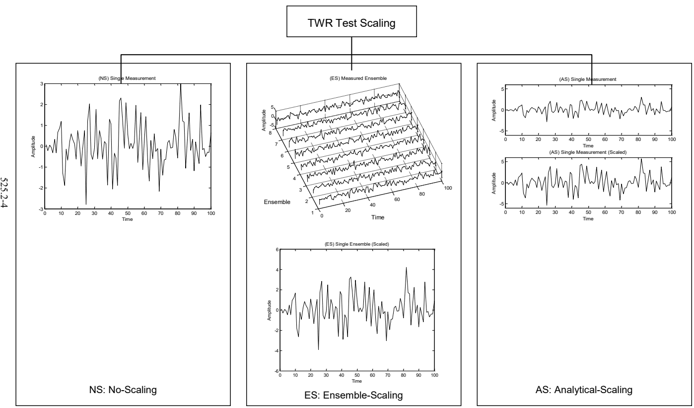
Figure description:
TWR Test Scaling 525.2-4
(NS Single Measurement
| Time | Amplitude |
|---|---|
| 0 | -0.2 |
| 10 | 1.2 |
| 20 | -0.5 |
| 25 | -2.8 |
| 30 | 0.8 |
| 40 | 0.2 |
| 45 | 2.3 |
| 50 | 0.5 |
| 60 | 2.0 |
| 70 | -2.2 |
| 80 | 0.8 |
| 82 | 3.0 |
| 90 | -1.2 |
| 100 | 0.0 |
(ES Measured Ensemble
| Time | Ensemble 1 | Ensemble 2 | Ensemble 3 | Ensemble 4 | Ensemble 5 | Ensemble 6 | Ensemble 7 | Ensemble 8 |
|---|---|---|---|---|---|---|---|---|
| 0 | 0.0 | -0.5 | 0.5 | -0.5 | 0.0 | 0.5 | -0.5 | -1.0 |
| 20 | -1.0 | 0.5 | -0.5 | 2.0 | 1.0 | -1.0 | 1.5 | 2.5 |
| 40 | 2.5 | -1.0 | 1.5 | -1.5 | 0.5 | 2.5 | -1.5 | -0.5 |
| 60 | -0.5 | 2.0 | -1.0 | 3.0 | -1.0 | -0.5 | 2.5 | 2.8 |
| 80 | 1.5 | -0.5 | 2.5 | 0.0 | 1.5 | 1.0 | -0.5 | -1.2 |
| 100 | -0.2 | 1.0 | -0.5 | 1.2 | -0.5 | 0.0 | 1.0 | 0.5 |
(ES Single Ensemble (Scaled
| Time | Amplitude |
|---|---|
| 0 | 0.0 |
| 10 | 1.7 |
| 12 | -2.6 |
| 20 | 0.5 |
| 25 | -3.8 |
| 30 | 2.7 |
| 40 | -3.0 |
| 50 | 3.2 |
| 60 | 2.8 |
| 70 | -2.8 |
| 82 | 4.2 |
| 90 | -1.5 |
| 100 | 0.0 |
(AS Single Measurement
| Time | Amplitude |
|---|---|
| 0 | 0.5 |
| 10 | -0.5 |
| 20 | 1.2 |
| 25 | -1.8 |
| 30 | 0.5 |
| 40 | 1.0 |
| 45 | -2.8 |
| 50 | 1.5 |
| 60 | 2.0 |
| 70 | -0.5 |
| 80 | 0.2 |
| 82 | 3.2 |
| 90 | -1.5 |
| 100 | 0.5 |
(AS Single Measurement (Scaled
| Time | Amplitude |
|---|---|
| 0 | 0.5 |
| 10 | 2.2 |
| 12 | -3.5 |
| 20 | 1.2 |
| 25 | -5.0 |
| 28 | 3.8 |
| 40 | 0.5 |
| 42 | 4.5 |
| 55 | -4.0 |
| 82 | 5.8 |
| 100 | 0.5 |
Notes: The figure illustrates three scaling methods for Time Waveform Replication (TWR tests: No-Scaling (NS, Ensemble-Scaling (ES, and Analytical-Scaling (AS. Each method's effect on single or ensemble measurements of amplitude over time is shown.))))
METHOD 525.2
MIL-STD-810H
|
Figure 525.2-1. Basic TWR test modes as related to time trace scaling.
MIL-STD-810H METHOD 525.2
1.2.6 General TWR Test Philosophy With Regard To Time Trace Simulation (and Scaling)
As emphasized in paragraph 1.2.4, time trace scaling to enhance conservativeness of laboratory testing is generally outside the scope of this Method. Figure 525.2-2 defines simulation possibilities within TWR including time trace scale rationale assumed to be provided external to this Method.
Two terms important to understanding TWR simulation will be introduced. The first term, intrinsic statistics, refers to the time-varying statistical estimates available from a single measured time trace (generally from short-time estimates). A single time trace has a confidence coefficient of 0.50, and the time-varying statistical estimates provide no information relative to the underlying ensemble-based random process, except for an estimate of the mean of the underlying random process. The second term, extrinsic statistics, refers to the time-varying statistical estimates available from more than one measured time trace, which forms a sample time trace ensemble. In this case, not only is an estimate of the underlying random process mean available, but also an estimate of its variance on a time increment basis. For comprehensive LCEP directed TWR materiel testing specifying analytical time traces through simulation, knowledge of the extrinsic statistics is essential. In general, specifying analytical time traces through simulation based upon intrinsic statistics is very limited, and usually unreliable for testing to the underlying random process (Method 519.8, Annex B discusses this further). Conversely, if a very small measured time trace sample ensemble is available, estimates of the underlying random process parameters tend to have large errors providing for an unreliable simulation. In this latter case, a more optimum test scenario is provided by replication of each of the individual measured time traces in a pre-defined sequence. A useful way to view intrinsic versus extrinsic statistics is to envision a One-Way Analysis of Variance, whereby the intrinsic statistics correspond to the “error within”, and the extrinsic statistics correspond to the “error among”.
Figure 525.2-2 attempts to clarify simulation issues for the four potential TWR test modes provided in the Figure. Whenever simulation is undertaken, it is implicit that the measured time trace(s) is scaled as a result of the simulation. This scaling is not considered “ad hoc” per se. The left most portion of the figure provides the simplest TWR test scenario with a single measured time trace and no scaling NS and no simulation (termed SM for Single-Measured). The left center portion of the figure provides for a single measured time trace with intrinsic trace time-average estimation used for creation of a simulated ensemble consisting of a single time trace, where AS is implied (termed SS for Single-Simulated). The right center portion provides the case of multiple measurements from a single phenomenon, with ensemble creation followed by simulation based upon combined intrinsic/extrinsic statistics and ES implied (termed MS for Multiple-Scaled). The right-most portion of the figure provides the case of multiple measurements from a single phenomenon, and the possibility of concatenation of the measurements (assuming ensemble information for simulation is too limited) (termed MM for Multiple-Measured). For generality, MM may allow for (but does not recommend) the use of “ad hoc” scaling of the individual measurements to be concatenated. To summarize, (1) SM is the recommended basic fully tailored TWR testing that this Method is designed to address; (2) SS is a less desired approach to replication of details of a single time trace with a minimal set of information that implies scaling a single time trace; (3) MS is recommended as a specialized information/labor intensive, but faithful approach to replication of an underlying random process under TWR and, finally, (4) MM is recommended for a time trace concatenation form of testing where “ad hoc” scaling procedures are best not applied.
|
It is vitally important that the distinctions made in Figure 525.2-1 and Figure 525.2-2 be recognized in TWR testing. In addition it is important to note the following:
- a. For zero mean Gaussian distributed stationary time traces, scaling is upon the random component alone, and ways of performing scaling for more than one time trace are provided in Method 519.8, Annex A. For these time traces, the statistics in the frequency domain, i.e., autospectral density estimates, are computed and envelopes determined.
- b. For time traces with a time-varying mean-square, it is unlikely that the ensemble representation of the underlying random process will have a time invariant or constant variance. If the underlying random process has a time-varying variance, then the sample time traces cannot be scaled by a constant and still preserve the probabilistic structure of the process.
Test TWR Simulation / Scaling
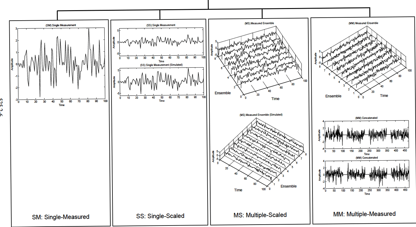
Figure description:
Comparison of Single-Measured, Single-Scaled, Multiple-Scaled, and Multiple-Measured Signal Processing Experimental vs. Simulated signal analysis across different data acquisition configurations
(SM Single Measurement
| Time | Amplitude |
|---|---|
| 0 | 0.0 |
| 10 | -1.2 |
| 20 | -2.5 |
| 30 | -0.7 |
| 40 | -0.5 |
| 50 | -0.2 |
| 60 | -1.5 |
| 70 | -0.4 |
| 80 | 2.8 |
| 90 | -0.6 |
| 100 | 0.5 |
(SS Single Measurement
| Time | Amplitude |
|---|---|
| 0 | 0.5 |
| 10 | 1.2 |
| 20 | -2.0 |
| 30 | 0.8 |
| 40 | 3.2 |
| 50 | -0.5 |
| 60 | 1.5 |
| 70 | -1.8 |
| 80 | 2.9 |
| 90 | 0.2 |
| 100 | -1.5 |
(SS Single Measurement (Simulated
| Time | Amplitude |
|---|---|
| 0 | 0.3 |
| 10 | 1.0 |
| 20 | -1.8 |
| 30 | 1.2 |
| 40 | 3.0 |
| 50 | -0.2 |
| 60 | 1.8 |
| 70 | -2.0 |
| 80 | 2.5 |
| 90 | 0.5 |
| 100 | -0.8 |
(MS Measured Ensemble
| Ensemble | Time | Amplitude |
|---|---|---|
| 1 | 0 | 0.0 |
| 1 | 50 | 2.5 |
| 1 | 100 | -1.0 |
| 4 | 0 | 0.5 |
| 4 | 50 | -1.5 |
| 4 | 100 | 2.0 |
| 8 | 0 | -1.2 |
| 8 | 50 | 3.0 |
| 8 | 100 | 0.2 |
(MS Measured Ensemble (Simulated
| Ensemble | Time | Amplitude |
|---|---|---|
| 1 | 0 | 0.2 |
| 1 | 50 | 2.0 |
| 1 | 100 | -0.8 |
| 4 | 0 | 0.3 |
| 4 | 50 | -1.2 |
| 4 | 100 | 1.8 |
| 8 | 0 | -1.0 |
| 8 | 50 | 2.8 |
| 8 | 100 | 0.5 |
(MM Measured Ensemble
| Ensemble | Time | Amplitude |
|---|---|---|
| 1 | 0 | -0.5 |
| 1 | 50 | 3.2 |
| 1 | 100 | -1.5 |
| 4 | 0 | 1.0 |
| 4 | 50 | -2.0 |
| 4 | 100 | 2.5 |
| 8 | 0 | -0.8 |
| 8 | 50 | 3.5 |
| 8 | 100 | 0.0 |
(MM Concatenated (Top
| Time | Amplitude |
|---|---|
| 0 | 0.0 |
| 50 | 1.8 |
| 100 | -2.2 |
| 150 | 1.5 |
| 200 | -0.5 |
| 250 | 2.5 |
| 300 | -1.8 |
| 350 | 1.0 |
| 400 | -2.5 |
| 450 | 2.2 |
(MM Concatenated (Bottom
| Time | Amplitude |
|---|---|
| 0 | -0.5 |
| 50 | 2.1 |
| 100 | -1.8 |
| 150 | 1.2 |
| 200 | -1.0 |
| 250 | 2.8 |
| 300 | -2.2 |
| 350 | 1.5 |
| 400 | -3.0 |
| 450 | 1.8 |
Notes: The figure showcases signal measurements and simulations across four different paradigms: Single-Measured (SM, Single-Scaled (SS, Multiple-Scaled (MS, and Multiple-Measured (MM. MS and MM include 3D waterfall plots of ensemble data.))))
METHOD 525.2
525.2-
MIL-SID-810H
Figure 525.2-2. Basic TWR test simulation combinations.
- c. For multiple time traces from the same underlying random process, creation of an ensemble may not be straight forward since it is nearly impossible to obtain measured time traces with exactly the same length by repeating the experiment, i.e., collection process (see paragraph 6.1, reference c.). It is also important to remember that the measured time traces must be “registered” or “serially correlated” according to some physical phenomenon, so that averaging over the ensemble members for each sample time point is meaningful. In the case where a valid ensemble is available, it is possible to estimate both the mean and variance of the random process at each time increment by averaging over the ensemble members. Under these circumstances, TWR testing could proceed on the basis of use of (a) the ensemble mean, (b) the “maximum” of the ensemble members, (c) all ensemble members, or (d) the ensemble mean plus (minus) a proportion of the square root of the ensemble variance. All four of these choices will preserve the probability structure of the unknown random process underlying the ensemble realizations. It is vitally important to note that “scaling” the ensemble mean, or any ensemble member by a constant factor, in general, will not provide time traces that are representative of the probability structure of the random process, unless the variance of the unknown random process is constant in time. Use of (d) above for TWR testing needs further amplification. The variance estimate obtained from averaging over the ensemble at each time increment will provide an unbiased estimate of the variance at the time increment with substantial random error or variation. Scaling each time point by the square root of the variance (with appropriate sign) provides for a “non-linear” transformation of the scaled time trace (since adjacent time increments may be scaled by factors that are different by an order of magnitude). Thus it becomes necessary to smooth the ensemble variance estimate in time to obtain acceptable time-varying scale factors. This smoothing introduces bias error with the benefit of decreased random error or variability. Unfortunately, there is little concrete guidance on the degree of smoothing that should be applied and, in fact, this becomes a form of a non-linear regression problem (i.e., smoothing is dependent upon the true unknown shape of the data being smoothed). Scaling based upon statistical ensemble estimates should only be performed by a competent data analyst familiar with random process theory, and the techniques of non-linear regression.
This summarizes the rationale behind the philosophy of this Method of simulation, and not directly recommending the “scaling” of measured time traces. Method 519.8, Gunfire Shock, Annex B, discusses extensively scaling for measured gunfire time traces.
In TWR testing involving analytically-specified deterministic time trace information, there is substantial test flexibility depending upon the assumptions that are made, be they ad hoc or from some rational basis. In this case, this Method becomes merely a tool for replicating what is generated without regard for the assumptions behind the specification. Any rationale for scaling is again external to this Method.
1.3 Limitations
This Method addresses very general time-varying traces not necessarily identifiable with underlying stationary or non-stationary random processes. It is apparent from various vendor TWR hardware/software configurations that the only requirement for application of this Method is the band-limited character of the time trace for replication, and its compatibility with the band-limited characteristics of the device (exciter) to be driven with the TWR hardware/software. For example, measured time traces that vary in frequency can be replicated as long as the time trace bandwidth is limited to overall bandwidth of the exciter control system. Non-Gaussian time traces can be replicated under TWR. All measured time traces can be replicated under TWR, provided they are within the band limit capabilities of the exciter control system to which they are applied for testing purposes. Limitations of this Method include the following:
- a. Does not address very long (several hour) time traces that can be termed “stationary” in nature (Gaussian or non-Gaussian and possibly have significant discrete components e.g., UAV measured environments). It is possible to repeat a given time trace multiple times, however, variations associated with actual experiment repetitions in the field will not be captured. It is important to note that, given a single stationary Gaussian or non-Gaussian time trace of sufficient length, it is possible to (1) divide this time trace into multiple time trace segments at zero crossings (required close to zero mean for each segment) and, (2) randomly place these segments into a permuted order to generate multiple time traces of sufficient length but essentially “stochastically independent” of one another. This can be particularly attractive for measured stationary non-Gaussian environments where the non-Gaussian “exact moment structure” must be preserved over long periods of time. The alternative to this is precise modeling of the measurement time trace and subsequent stochastic generation of unlimited segments for TWR input.
MIL-STD-810H
METHOD 525.2
- b. Does not address the advantages and disadvantages of replicating very short duration time traces (shocks) over and above application of Method 516.8.
- c. Does not explicitly address time traces that have highly variable frequency characteristics in time.
- d. Does not explicitly address time traces that are nonlinear in nature.
- e. Does not explicitly address repeated environments that may be of a non-stationary nature because of the occurrence pattern of the environment. For example, no discussion is provided on occurrence statistics that may be modeled in terms of a non-stationary (rate-varying) Poisson process.
- f. Generally does not address the characteristics of the time trace on the materiel in terms of materiel "rise-time" response.