In addition to the guidance provided in Part One, paragraphs 5.14 and 5.17; and Part One, Annex A, Tasks 405 and 406, the following information is provided to assist in the evaluation of the test results. Analyze in detail any failure of a test item to meet the requirements of the specification, and consider related information such as:
- a. Information from the control accelerometer configuration, including a digital record of the control time trace.
- b. The vendor TWR software test tolerance information.
- c. Application of one or more of the techniques illustrated in Annex A and elaborated on in Annex B for detailed comparison of the reference time trace to the control time trace.
525.2-5 POST-TEST PROCESSING FOR TPP
From pre-processing, three individual segments of different form exist along with the overall time trace. For reference purposes, the overall difference time trace along with TPP root-mean-square level are displayed in Figures 525.2A- 9a and 525.2A-9b. In addition, the difference of the differences is provided in Figure 525.2A-9c.
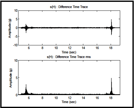
Figure description:
Time Trace Analysis of s(H Difference
s(H : Difference Time Trace
| Time (sec) | Amplitude (g) |
|---|---|
| 4.5 | 0.0 |
| 5.0 | 0.2 |
| 5.3 | 0.4 |
| 5.5 | 1.8 |
| 5.6 | -2.9 |
| 5.7 | 1.5 |
| 6.0 | 0.3 |
| 8.0 | -0.1 |
| 10.0 | 0.1 |
| 12.0 | -0.2 |
| 14.0 | 0.1 |
| 16.0 | -0.1 |
| 17.5 | 0.3 |
| 18.0 | -1.5 |
| 18.1 | 4.8 |
| 18.2 | -4.2 |
| 18.5 | 0.5 |
| 19.5 | 0.0 |
s(H : Difference Time Trace rms
| Time (sec) | Amplitude (g) |
|---|---|
| 4.5 | 0.1 |
| 5.0 | 0.3 |
| 5.4 | 1.0 |
| 5.5 | 2.5 |
| 5.6 | 3.1 |
| 6.0 | 0.5 |
| 8.0 | 0.2 |
| 10.0 | 0.3 |
| 12.0 | 0.2 |
| 14.0 | 0.3 |
| 16.0 | 0.2 |
| 17.5 | 0.5 |
| 18.0 | 1.2 |
| 18.1 | 4.9 |
| 18.2 | 1.8 |
| 18.5 | 0.4 |
| 19.5 | 0.1 |
Notes: The signal shows two distinct bursts of vibration amplitude at approximately 5.6 seconds and 18.1 seconds. The first burst has an RMS peak of approximately 3.1g, while the second burst is stronger with an RMS peak of approximately 4.9g.
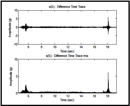
Figure description:
Comparison of Difference Time Trace and its RMS Value
s(S : Difference Time Trace
| Time (sec) | Amplitude (g) |
|---|---|
| 4.0 | 0.0 |
| 4.5 | 0.1 |
| 5.0 | 0.8 |
| 5.2 | -1.0 |
| 5.5 | 2.2 |
| 5.6 | -2.4 |
| 5.8 | 1.5 |
| 6.0 | 0.2 |
| 8.0 | 0.1 |
| 10.0 | 0.3 |
| 12.0 | 0.2 |
| 14.0 | 0.4 |
| 16.0 | 0.1 |
| 17.5 | 0.4 |
| 18.0 | 1.0 |
| 18.1 | 6.1 |
| 18.2 | -4.2 |
| 18.5 | 0.1 |
| 19.0 | 0.0 |
s(S : Difference Time Trace rms
| Time (sec) | Amplitude (g) |
|---|---|
| 4.0 | 0.1 |
| 4.5 | 0.2 |
| 5.0 | 1.0 |
| 5.2 | 1.2 |
| 5.5 | 2.3 |
| 5.6 | 2.7 |
| 5.8 | 1.8 |
| 6.0 | 0.5 |
| 8.0 | 0.3 |
| 10.0 | 0.5 |
| 12.0 | 0.4 |
| 14.0 | 0.6 |
| 16.0 | 0.2 |
| 17.5 | 0.5 |
| 18.0 | 1.2 |
| 18.1 | 6.2 |
| 18.5 | 0.2 |
| 19.0 | 0.1 |
Notes: The charts display vibration data (amplitude in g over time. The top chart shows the raw difference time trace, while the bottom chart shows the root-mean-square (rms version of the same signal. Two distinct bursts of activity are visible: one around 5.5-5.8 seconds and a larger one around 18.1 seconds.))
Figure 525.2A-9a. Difference Exciter (H).
Figure 525.2A-9b. Difference Exciter (S).
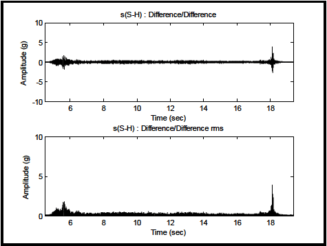
Figure description:
Vibration Analysis Signals
s(S-H : Difference/Difference
| Time (sec) | Amplitude (g) |
|---|---|
| 4.5 | 0.1 |
| 5.0 | -0.1 |
| 5.2 | 0.3 |
| 5.3 | 0.8 |
| 5.4 | -1.5 |
| 5.5 | 1.8 |
| 5.6 | -1.7 |
| 5.7 | 1.4 |
| 5.8 | -0.9 |
| 6.0 | 0.2 |
| 7.0 | -0.1 |
| 8.0 | 0.1 |
| 9.0 | -0.1 |
| 10.0 | 0.1 |
| 11.0 | -0.1 |
| 12.0 | 0.1 |
| 13.0 | -0.1 |
| 14.0 | 0.1 |
| 15.0 | -0.1 |
| 16.0 | 0.1 |
| 17.0 | -0.2 |
| 17.5 | 0.4 |
| 17.8 | -0.8 |
| 17.9 | 0.6 |
| 18.0 | -1.2 |
| 18.1 | 4.0 |
| 18.2 | -2.5 |
| 18.3 | 0.8 |
| 18.5 | -0.4 |
| 19.0 | 0.1 |
| 19.5 | 0.0 |
s(S-H : Difference/Difference rms
| Time (sec) | Amplitude (g) |
|---|---|
| 4.5 | 0.1 |
| 5.0 | 0.4 |
| 5.2 | 0.8 |
| 5.3 | 1.2 |
| 5.4 | 1.5 |
| 5.5 | 1.9 |
| 5.6 | 1.7 |
| 5.7 | 1.3 |
| 5.8 | 0.8 |
| 6.0 | 0.6 |
| 7.0 | 0.3 |
| 8.0 | 0.3 |
| 9.0 | 0.2 |
| 10.0 | 0.2 |
| 11.0 | 0.2 |
| 12.0 | 0.3 |
| 13.0 | 0.2 |
| 14.0 | 0.3 |
| 15.0 | 0.2 |
| 16.0 | 0.2 |
| 17.0 | 0.4 |
| 17.5 | 0.6 |
| 17.8 | 0.7 |
| 17.9 | 0.9 |
| 18.0 | 1.4 |
| 18.1 | 4.0 |
| 18.2 | 1.1 |
| 18.3 | 0.6 |
| 18.5 | 0.4 |
| 19.0 | 0.1 |
| 19.5 | 0.1 |
Notes: The figure consists of two time-series plots. The first plot displays the raw difference signal, which fluctuates around a zero baseline with distinct bursts of high-amplitude activity. The second plot shows the Root Mean Square (RMS of this signal, highlighting the energy level of the vibration events over the same time period.)
Figure 525.2A-9c. Time Trace of Difference of the Differences ((S) - (H)).
Figures 525.2A-9a-9c. Plots of overall difference time trace with root-mean-square.
In this particular case, TPP difference s(H) and s(S) may approach 5g, whereby the reference time trace was bounded by 40g in the positive and negative directions. This would suggest that, in certain parts of the time trace, the normalized random error might approach 0.125, i.e., 12.5 percent. The rudimentary overall maximum and minimum statistics for the time traces are as follows: r(H) min/max -22.84/35.24; c(H) min/max -24.28/39.76; and s(H) min/max -4.11/4.78; c(S) min/max -23.85/39.03; and s(S) min/max -3.95/6.08. The differences between response on the head of the shaker (H) and the shaker slip table (S) are reasonably nominal, so that only results for the shaker head will be provided below. When reviewing several test measurements, it is usually desirable to provide comprehensive post-test analysis on one set of measurements, and infer that similar analysis on the other measurements. The segments will now be processed in turn according to meaningful and easy to interpret estimates.
MIL-STD-810H METHOD
5.1 Physics of Failure
Analyses of vibration related failures must relate the failure mechanism to the dynamics of the failed item and to the dynamic environment. It is insufficient to determine that something failed due to high cycle fatigue or wear. Include in failure analyses a determination of resonant mode shapes, frequencies, damping values and dynamic strain distributions, in addition to the usual material properties, crack initiation locations, etc.
5.2 Qualification Tests
When a test is intended to show formal compliance with contract requirements, recommend the following definitions:
- a. Failure definition. Materiel is deemed to have failed if it suffers permanent deformation or fracture; if any fixed part or assembly loosens; if any moving or movable part of an assembly becomes free or sluggish in operation; if any movable part or control shifts in setting, position or adjustment, and if test item performance does not meet specification requirements while exposed to operational or endurance test levels. Ensure this statement is accompanied by references to appropriate specifications, drawings, and inspection methods.
MIL-STD-810H
METHOD 525.2
- b. Test completion. A TWR qualification test is complete when all elements of the test item have successfully passed a complete test. When a failure occurs, stop the test, analyze the failure and repair the test item. Continue the test until all fixes have been exposed to a complete test. Qualified elements that fail during extended tests (tests extended beyond LCEP requirements) are not considered failures, and can be repaired to allow test completion.
5.3 Other Tests
For tests other than qualification tests, prepare success and/or failure criteria and test completion criteria that reflect the purpose of the tests.