The expected duration of vibration exposure is derived from the system’s mission or lifetime scenario, often provided in the LCEP. A system’s mission or lifecycle scenario is a key parameter for a VSD effort. In some cases a number of mission types are required, each with differing proportions of terrain or maneuvers utilized. These must all be weighted appropriately depending upon the user requirement/LCEP and used in the generation of the vibration schedule. As a minimum, the scenario for a ground vehicle must provide terrain type, average and maximum speeds associated with each terrain type, and total distance traveled on each terrain type. For an aircraft, the scenario must provide a detailed description of all flight conditions, including hover, forward level flight, take-off/ landing and other and relevant maneuvers. The description should include the percentage of flight duration represented by each condition and the number of repetitions for each maneuver.
514.8-7 COMBINING LVTS
It is sometimes necessary to combine multiple LVTS into one. This can be due to the need to combine the exposure of more than one vehicle, or the desire to combine multiple LVTS developed for a single vehicle. For ASD's with similar spectral shapes, the following method can be used to combine the broadband portions of two or more LVTS. Refer to Table 514.8F-D.IX for an example of the calculations for combining two LVTS, LVTS01 and LVTS02. Note that each LVTS will consist of an ASD and an associated runtime. For the example assume LVTS01 Runtime = 30 min; LVTS02 Runtime = 15 min; Final Runtime = 20 min. First, Miner's Rule is utilized to perform a spectral line-by spectral line scaling of each LVTS to some normalized level. In the example each spectral line is normalized to the value of LVS02. This process assigns new test times to each spectral line of each LVTS. Once the power levels of the LVTS are equated, the individual times can simply be totaled on a spectral line basis. At this point a new combined LVTS has been created, LVTS_C. However, each spectral line has a varying associated test time. For the final step, the levels for each spectral line are scaled using Equation 9-5 such that all spectral lines are normalized to a final runtime selected by the analyst. A similar approach can be utilized to combine narrowbands or sine tones.
MIL-STD-810H
METHOD 514.8, ANNEX F, APPENDIX D
| Freq | LVTS01 | LVTS02 | Norm Level | LVTS01 New Time | LVTS02 New Time | Total New Time | Final Run Time | LVTS_C |
|---|---|---|---|---|---|---|---|---|
| (Hz) | (G²/Hz) | (G²/Hz) | (G²/Hz) | (min) | (min) | (min) | (min) | (G²/Hz) |
| 5 | 0.100 | 0.200 | 0.200 | 2.23 | 15.00 | 17.23 | 20.00 | 0.208 |
| 6 | 0.200 | 0.400 | 0.400 | 2.23 | 15.00 | 17.23 | 20.00 | 0.415 |
| 7 | 0.300 | 0.400 | 0.400 | 10.20 | 15.00 | 25.20 | 20.00 | 0.459 |
| 8 | 0.400 | 0.400 | 0.400 | 30.00 | 15.00 | 45.00 | 20.00 | 0.536 |
| 9 | 0.400 | 0.300 | 0.300 | 88.24 | 15.00 | 103.23 | 20.00 | 0.501 |
This method can also be used this to combine multiple events into a broadband LVTS, replacing the steps outline in paragraphs 2.6 through 2.8 above. An alternate method to add conservatism must be found, and care should be taken to assure the method does not corrupt the overall shape of the ASD set. Refer to paragraph 2.2.1 (main body of Method 514) for cautions associated with combining LVTS.
Downloaded from https://www.everyspec.com
MIL-STD-810H
METHOD 514.8, ANNEX F, APPENDIX D
(This page is intentionally blank.)
MIL-STD-810H METHOD 514.8, ANNEX F, APPENDIX E METHOD 514.8, ANNEX F, APPENDIX E Theoretical Aspects of Maximum Response
7.1 Ground Vehicle
Often, scenario information in the form required for the VSD process is not available. This is particularly true for vehicles not yet in the DoD inventory. If no information is available the scenario information may be inferred by the intended usage. For cargo items, the ground distance is determined based upon transport distance between each of the designated supply points that extend from the depot through the Port Staging Area (PSA) to the user of the item. For installed equipment items, the ground distance is determined on the basis of the maintenance schedule for the
MIL-STD-810H
vehicle on which the equipment is mounted or on the basis of designer/user agreed upon repair/replacement schedule for the particular installed equipment item.
Often, limited scenario information can be found in the vehicles LCEP or other documentation. This information typically includes overall terrain type distance percentages and sometimes includes total distance and maximum and/or average speed information. Extensive manipulation is often required to distribute the total distance into the various road surfaces and speeds that characterize the vehicles usage. This process is illustrated in Table 514.8F-I.
The Level 1 breakout of Table 514.8F-I contains the minimum scenario information required for a VSD. The Level 2 breakout is a distribution of the general terrain type mileage into the various test surfaces for which data is typically acquired. All surfaces likely to be encountered for a given terrain type should be included in the Level 2 breakout. Surfaces used for Department of Defense (DoD) projects should be similar to those listed in Table 514.8F-I and described in reference r. Level 2 breakout information is rarely available and is typically derived through discussion between the analyst, the user, and other interested parties.
MIL-STD-810H
METHOD 514.8, ANNEX F
| LEVEL 1 BREAKOUT | LEVEL 2 BREAKOUT | ||||||||
|---|---|---|---|---|---|---|---|---|---|
| TOTAL MILES: | 1000 | ||||||||
| Terrain Type | Percent | Miles | Speed | Surface¹ | Percent | Miles | Speed | ||
| Max | Avg | Max | Avg | ||||||
| PRIMARY ROAD | 70% | 700 | 55 | 35 | Paved | 100% | 700 | 55 | 35 |
| 100% | 700 | ||||||||
| SECONDARY ROAD | 20% | 200 | 40 | 22 | Secondary Road | 60% | 120 | 40 | 25 |
| Gravel Road | 23% | 46 | 45 | 22 | |||||
| Belgian Block | 10% | 20 | 25 | 15 | |||||
| Embedded Rock | 1% | 2 | 10 | 7 | |||||
| Radial Washboard | 3% | 6 | 15 | 9 | |||||
| 2" Washboard | 3% | 6 | 10 | 7 | |||||
| 100% | 200 | ||||||||
| * Off Road | 10% | 100 | 25 | 14 | Cross Country | 85% | 85 | 25 | 16.3 |
| * A combination of trails and cross country | Embedded Rock | 5% | 5 | 10 | 7 | ||||
| Radial Washboard | 5% | 5 | 15 | 9 | |||||
| 2" Washboard | 5% | 5 | 10 | 7 | |||||
| 100% | 100 | ||||||||
| LEVEL 1 | This information should be provided by the program manager and is required before LVTS development can begin. This information can sometimes be found in the LCEP or other system documentation. | ||||||||
| LEVEL 2 | This breakout has a significant impact on the test durations of the final LVTS and should therefore be given serious consideration. This information, too, should be provided but is seldom available. Development cannot begin without this breakout. Often the analyst is forced to recommend a breakout for the concurrence of user. | ||||||||
MIL-STD-810H METHOD 514.8, ANNEX F
7.1.1 Beta Distribution
Once consensus is reached on the Level 2 breakout, the distance must be further distributed into the various speeds for which data was acquired. This additional level of fidelity is rarely provided. One option is to utilize the Beta distribution to distribute surface distance into the speed events for that surface. The Beta is a probability distribution with two shaping parameters, and , calculated as defined in equation 7.1 where x is the normalized distribution range.
f(x) = (a + B-1)! -xa-1 (1-x) B-1 (7.1) (a-1)!(B-1)!
Guidelines have been established to allow consistent selection of and , based on the ratio of the average to maximum speed. Alpha can be selected from Table 514.8F-II. Beta is iteratively calculated to yield a calculated average speed from the Beta distribution results to match the average speed provided in the scenario. The Beta distribution should be utilized to distribute the distance into a set of speed ranges, rather than into a set of discreet speeds. An alternative to distributing the total distance is to distribute the total time, based on the total distance and average speed. A Beta distribution is produced for each road surface utilizing a spreadsheet. An example Beta distribution spreadsheet is provided in Figure 514.8F-1.
Table 514.8F-II: Selection of Alpha for Beta Distribution
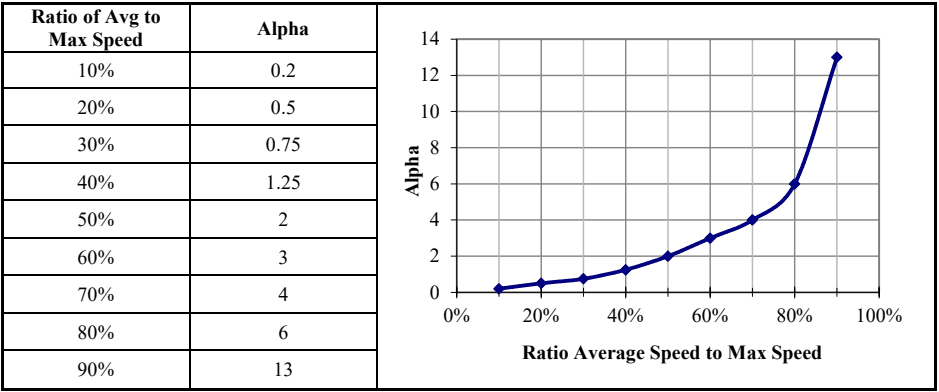
Figure description:
Legend
- Alpha — color: Dark blue; symbol: Line with diamond markers
| Ratio of Avg to Max Speed | Alpha |
|---|---|
| 10% | 0.2 |
| 20% | 0.5 |
| 30% | 0.75 |
| 40% | 1.25 |
| 50% | 2 |
| 60% | 3 |
| 70% | 4 |
| 80% | 6 |
| 90% | 13 |
Notes: The image displays a data table and its corresponding line graph showing the relationship between the ratio of average speed to maximum speed and the parameter Alpha. The graph shows an exponential-like increase in Alpha as the ratio approaches 100%.
MIL-STD-810H
METHOD 514.8, ANNEX F
| BETA DISTRIBUTION INPUTS | |
|---|---|
| SURFACE | Paved Road |
| MIN SPEED OF DATA SET | 5 |
| MAX SPEED OF DATA SET | 55 |
| AVG SPEED FROM SCENARIO | 35 |
| SPEED INCREMENT OF DATA SET | 5 |
| TOTAL MILES FROM SCENARIO | 700.00 |
| TOTAL HOURS | 20.000 |
| Ratio Avg/Max Speed | 64% |
| CALCULATED RESULTS | |
|---|---|
| Dist Min Speed | 0 |
| Dist Max Speed | 57.5 |
| ALPHA | 3.40 |
| BETA | 2.19 |
| Average Speed | 35.00 |
| Total Miles | 699.982 |
| Total Hours | 20.000 |
| Error | 0.00% |
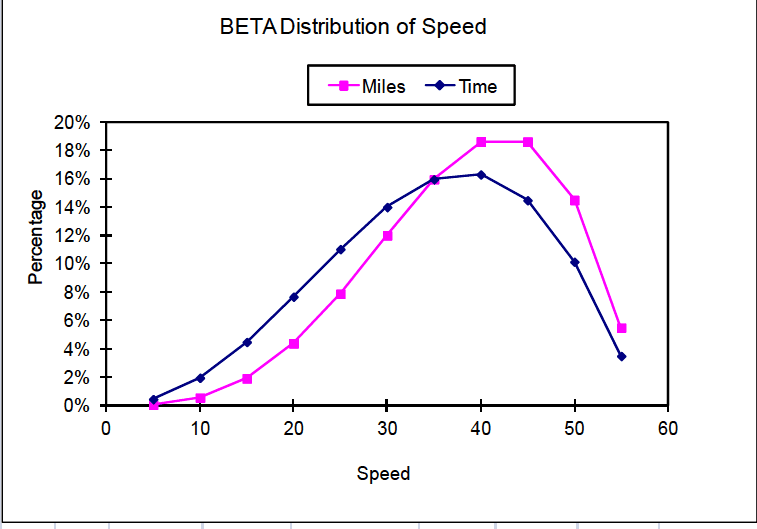
Figure description:
BETA Distribution of Speed
BETA Distribution of Speed
Legend
- Miles — color: magenta; symbol: Solid line with square marker
- Time — color: dark blue; symbol: Solid line with diamond marker
| Speed | Miles (Percentage) | Time (Percentage) |
|---|---|---|
| 5 | 0.1% | 0.4% |
| 10 | 0.5% | 2.0% |
| 15 | 1.9% | 4.5% |
| 20 | 4.3% | 7.6% |
| 25 | 7.8% | 11.0% |
| 30 | 12.0% | 14.0% |
| 35 | 15.9% | 16.0% |
| 40 | 18.6% | 16.3% |
| 45 | 18.6% | 14.5% |
| 50 | 14.5% | 10.1% |
| 55 | 5.5% | 3.5% |
| BETA DISTRIBUTION OF SPEED | ||||||||
|---|---|---|---|---|---|---|---|---|
| Repr | Start | End | Range | Percentage | Time | Percentage | ||
| Speed | Speed | Speed | Avg | Time | in Hours | in Min | Miles | Miles |
| n/a | 0 | 2.5 | 1.25 | 0.012% | 0.002 | 0.15 | 0.0031 | 0.00% |
| 5 | 2.5 | 7.5 | 5 | 0.458% | 0.092 | 5.50 | 0.46 | 0.07% |
| 10 | 7.5 | 12.5 | 10 | 1.966% | 0.393 | 23.59 | 3.93 | 0.56% |
| 15 | 12.5 | 17.5 | 15 | 4.487% | 0.897 | 53.84 | 13.46 | 1.92% |
| 20 | 17.5 | 22.5 | 20 | 7.673% | 1.535 | 92.08 | 30.69 | 4.38% |
| 25 | 22.5 | 27.5 | 25 | 11.035% | 2.207 | 132.42 | 55.18 | 7.88% |
| 30 | 27.5 | 32.5 | 30 | 13.999% | 2.800 | 167.99 | 84.00 | 12.00% |
| 35 | 32.5 | 37.5 | 35 | 15.955% | 3.191 | 191.46 | 111.68 | 15.95% |
| 40 | 37.5 | 42.5 | 40 | 16.295% | 3.259 | 195.54 | 130.36 | 18.62% |
| 45 | 42.5 | 47.5 | 45 | 14.478% | 2.896 | 173.74 | 130.31 | 18.62% |
| 50 | 47.5 | 52.5 | 50 | 10.142% | 2.028 | 121.71 | 101.42 | 14.49% |
| 55 | 52.5 | 57.5 | 55 | 3.499% | 0.700 | 41.99 | 38.49 | 5.50% |
| TOTAL | 100.0% | 20.000 | 1200.00 | 699.982 | 100.0% | |||
| TOTAL USED | 100.0% | 19.998 | 1199.85 | 699.979 | 100.0% | |||
Figure 514.8F-1. Sample beta distribution (wheeled vehicle).
The Beta distribution calculations are performed in the “BETA DISTRIBUTION OF SPEED” table of Figure 514.8F-1. A description of the fields follows.
- a. Repr Speed - The representative speed for this entry. This is the speed for which vibration data were acquired.
- b. Start Speed – The beginning of the speed range for this entry.
- c. End Speed – The ending of the speed range for this entry.
- d. Range Average – The average of the speed range for this entry. This number should be equal to the representative speed for the entry.
- e. Percentage Time – This is the actual Beta distribution as a percentage of the total drive time. This column, along with the Percentage Miles column, is plotted on the graph of Figure 514.8F-1.
- f. Time in Hours – The time in hours represented by this data entry, calculated by multiplying the total hours by the percentages of the previous column. The total hours is calculated from the total miles and the average speed.
- g. Time in Min. – The time in minutes represented by this data entry. This is the final output of the Beta distribution and is passed forward to the VSD process.
- h. Miles – The miles represented by this data entry, calculated by multiplying the Time in Hours by the Range Average.
- i. Percentage Miles – The percentage of the total miles represented by this entry. This column, along with the Percentage Time column, is plotted on the graph of Figure 514.8F-1.
Note that the widths (in units of speed) of each speed range in the table of Figure 514.8F-1 are equal to the speed increment for which data was acquired and are centered around the acquired speeds. This results in two slight inconsistencies at the endpoints of the Beta distribution. First, the percentage of the miles at very low speeds (below 2.5 mph in this example) is not included in the VSD process. It is expected that the vibration at these speeds will be quite low and have no effect on the resultant LVTS, even if included. Second, the maximum speed of the Beta distribution is one-half speed increment higher than the highest speed for which data was acquired. This too should have little effect on the VSD process since very little time is spent at this speed.
The endpoints of the Beta distribution technique are treated slightly different for NBROR or SOR LVTS. In those cases, the endpoints for Beta distribution are set to exactly the minimum and maximum speeds acquired. If the example presented here were for a tracked vehicle the range of the first entry would be from 5 to 7.5 mph instead of 2.5 to 7.5 mph. Likewise, the last entry would be from 42.5 to 45 mph instead of 42.5 to 47.5 mph. For a tracked vehicle the narrowband random sweeps dominate the fatigue exposure represented by an LVTS. The same is true for the swept sine LVTS. Therefore, more emphasis is placed on the sweep ranges when calculating the Beta distribution. The sweep ranges are bound by the frequencies associated with the minimum and maximum speeds acquired, and the Beta distribution ranges are selected to account for that. Note that the speed ranges of the endpoints are then one-half as wide as the intermediate points. This is accounted for in the VSD process when calculating the actual run time represented by each speed event. The run times of the first and last speeds are set to one half of the intermediate speeds. Note also that during testing on the shaker, the swept narrow bands are in the range of the endpoint speeds for one-half the time of the other speeds.
7.2 Aircraft
The scenario for cargo and installed equipment transported by aircraft is generally measured in time rather than distance. The time begins with the standby-engine running phase and progresses through ascent, level flight, maneuvers, and ends with descent and landing. It is imperative that the scenario information for a given aircraft provides sufficient flight conditions to adequately describe the most severe vibration environment. For example, level flight should include a range of speeds between minimum and maximum in order to determine the most severe level flight condition. In addition, the number of flights must be known so that the laboratory test time can be determined.
Detailed scenario information is generally more readily available for aircraft than for ground vehicles in the form of usage spectrums. A usage spectrum is a tabulation of the percentage of flight time associated with all maneuvers relevant for the aircraft. This information feeds directly into the tables required for VSD. Generally, the only manipulation required is to combine the usage of the extensive list of maneuvers included in an aircraft's usage
MIL-STD-810H
spectrum into the relatively few maneuvers for which data is typically acquired. During the data acquisition phase, it is typically not feasible to acquire data for all the maneuvers in an aircraft’s usage spectrum. Engineering judgment is exercised when selecting a representative set of maneuvers for which data is acquired, although it is common practice to explore the limits of the allowable aircraft flight envelope (altitude, speed, angle of attack, throttle variations, acceleration etc.) plus enough information to allow extrapolation/interpolation to cover other events. Likewise, the flight time percentages of all maneuvers in the usage spectrum must be distributed into the maneuvers for which data was acquired. This analysis should rely on sources knowledgeable of aircraft usage to assist in scenario development.
7.3 Sea Vehicle
Materiel installed aboard naval ships is subjected to varying frequencies and amplitudes of environmental vibration for extended periods of time, during which they are required to perform their normal function. Principal causes of steady state shipboard vibration are propeller blade excitation and unbalanced forces of the propeller and shafting. Vibrations are also experienced by shipboard mounted equipment caused by mounting system resonances, changes in ship speed and heading, and changes in sea state.
Equipment integrated onto a ship will generally have a much longer service life than that of cargo. For either case, one would expect the LCEP to consist of the number of hours at sea subdivided into various sea states. If an exact breakdown of sea states is not provided, an experienced analyst may take advantage of the Beta distribution techniques discussed in the previous section as a method of refining the LCEP.
7.4 Rail Transport
Material installed on railcars is primarily subjected to low level broadband vibration affected primarily by the railcar speed. There are no surface considerations. If an exact breakdown of speeds is not provided, an experienced analyst may take advantage of the Beta distribution techniques discussed in the previous section as a method of refining the LCEP.