517.3-2 ALIASED DATA
The data shown in Figure 517.3A-1 are a complex shock that starts with a near-field pyroshock followed by two mechanical shock events as shown in paragraph 6.1, reference r. The accelerometer used to measure these data is a piezoresistive type. These data were sampled at 25,000 Hz, and taken with a data acquisition system (DAS) that has an “anti-aliasing Bessel filter” that is - 3 dB at a 20,000 Hz cutoff frequency, as per manufacturer’s specifications. This specification means that the filter attenuation is only 80 dB down in a decade (200,000 Hz), and that the data are severely aliased. For example, the sample rate of 25,000 Hz gives a Nyquist frequency (highest frequency that can be resolved at the given sample rate) of 12,500 Hz. Consequently, the anti-aliasing filter provides no protection at all at this sample rate, or even at the higher sample rates of up to 100,000 Hz. The recommended practice for pyroshock data is an anti-aliasing filter that is 60 dB/octave, and the cutoff frequency should be at least one octave below the Nyquist frequency as per paragraph 6.1, references b, d, and f. The requirements of Paragraph 2.3.2 of this document are an equivalent way to achieve the same aliasing protection with more flexibility in other data parameters. Additionally, the recommended practice is to sample at least ten times higher than the desired bandwidth of the measurement in order to achieve 5% or less amplitude error as per paragraph 6.1, references b, d, and f.
The integral of the data shown in Figure 517.3A-1 is in Figure 517.3A-2. The velocity should start and end at zero because the materiel on which the data were taken starts in a stationary position, and is in that same position at the end of the complex shock. However, the velocity time history clearly shows the characteristics of aliasing as per paragraph 6.1, reference p.
MIL-STD-810H
METHOD
2.1 Selecting the Pyroshock Method
After examining requirements documents and applying the tailoring process in Part One of this Standard to determine where pyroshock effects are foreseen in the life cycle of the materiel, use the following to confirm the need for this Method and to place it in sequence with other Methods.
2.1.1 Effects of Pyroshock
In general, pyroshock has the potential for producing adverse effects on all electronic materiel. The level of adverse effects generally increases with the level and duration of the pyroshock, and decreases with the distance from the source (pyrotechnic device) of the pyroshock. Durations for pyroshock that produce material stress waves with wavelengths that correspond with the natural frequency wavelengths of microelectronic components within materiel will enhance adverse effects. In general, the structural configuration merely transmits the elastic waves and is unaffected by the pyroshock. Examples of problems associated with pyroshock follow, but the list is not intended to be all-inclusive.
- a. Materiel failure as a result of destruction of the structural integrity of micro-electronic chips.
- b. Materiel failure as a result of relay chatter.
- c. Materiel failure as a result of circuit card malfunction, circuit card damage, and electronic connector failure. On occasion, circuit card contaminants having the potential to cause short circuits may be dislodged under pyroshock.
MIL-STD-810H
METHOD 517.3
- d. Materiel failure as a result of cracks and fracture in crystals, ceramics, epoxies, or glass envelopes.
2.1.2 Sequence Among Other Methods
- a. General. Use the anticipated life cycle sequence of events as a general sequence guide (see Part One, paragraph 5.5).
- b. Unique to this Method. Unless otherwise displayed in the life cycle profile and, since pyroshock is normally experienced near the end of the life cycle, schedule pyroshock tests late in the test sequence. In general, the pyroshock tests can be considered independent of the other tests because of their unique nature.
2.2 Selecting a Procedure
NOTE: For materiel design and development, the option of tailoring of a laboratory shock test from field measurement information is superior to any of the test procedures within this Method, and should be the first laboratory test option. This assumes that the measurement data bandwidth and the laboratory test bandwidths are strictly compatible.
This Method includes five pyroshock test procedures:
- a. Procedure I - Near-field with an Actual Configuration. Replication of pyroshock for the near-field environment using the actual materiel, and the associated pyrotechnic shock test device configuration.
- b. Procedure II - Near-field with a Simulated Configuration. Replication of pyroshock for the near-field environment using the actual materiel, but with the associated pyrotechnic shock test device isolated from the test item, e.g., by being mounted on the back of a flat steel plate. (This normally will minimize testing costs because fewer materiel configurations and/or platforms associated with the test item will be damaged. This can be used for repeated tests at varying pyroshock levels.)
- c. Procedure III - Mid-field with a Mechanical Test Device. Replication of pyroshock for the mid-field environment with a mechanical device that simulates the pyroshock peak acceleration amplitudes and frequency content (other than an electrodynamic shaker because of frequency range and weight limitations of an electrodynamic shaker).
- d. Procedure IV - Far-field with a Mechanical Test Device. Replication of pyroshock for the far-field environment with a mechanical device that simulates the pyroshock peak acceleration amplitudes and frequency content (other than an electrodynamic shaker because of frequency range and weight limitations of an electrodynamic shaker).
- e. Procedure V - Far-field with an Electrodynamic Shaker. Replication of pyroshock for the far-field environment using an electrodynamic shaker to simulate the comparatively low frequency structural resonant response to the pyroshock.
2.2.1 Procedure Selection Considerations
Based on the test data requirements, determine which test procedure is applicable. In most cases, the selection of the procedure will be dictated by the actual materiel configuration, carefully noting any structural discontinuities that may serve to mitigate the effects of the pyroshock on the materiel. In some cases, the selection of the procedure will be driven by test practicality. Consider all pyroshock environments anticipated for the materiel during its life cycle, both in its logistic and operational modes. When selecting procedures, consider:
- a. The Operational Purpose of the Materiel. From the requirements documents, determine the functions to be performed by the materiel either during or after exposure to the pyroshock environment.
- b. The Natural Exposure Circumstances for Pyroshock. Determine if the materiel or portion of the materiel lies within the near-field, mid-field or far-field of the pyrotechnic device. Use Procedure I or II if the materiel or a portion of the materiel lies within the near-field of the pyrotechnic device, no special isolation of the materiel exists, or if there are no prior measured field data. Choose Procedure III, IV, or V based on the frequency content and amplitude of available data, as well as the limitations of the test device. In any case,
one test will be considered sufficient for testing over the entire amplitude and frequency range of exposure of the materiel. Do not break up any measured or predicted response to pyroshock into separate frequency ranges for the purpose of applying different testing procedures to different frequency ranges.
c. Required Data. The test data required to verify that the materiel will survive and function as intended.
2.2.2 Difference Among Procedures
- a. Procedure I - Near-field with Actual Configuration. Procedure I is intended to test materiel in its functional mode and actual configuration (materiel/pyrotechnic device physical configuration), and to ensure it can survive and function as required when tested using the actual pyrotechnic test device in its intended installed configuration. In Procedure I, it is assumed that the materiel or a portion of the materiel resides within the near-field of the pyrotechnic device.
- b. Procedure II - Near-field with Simulated Configuration. Procedure II is intended to test materiel in its functional mode, but with a simulated structural configuration, and to ensure it can survive and function as required when in its actual materiel/pyrotechnic device physical configuration. In this procedure it is assumed that some part of the materiel lies within the near-field. Make every attempt to use this procedure to duplicate the actual platform/materiel structural configuration by way of a full-scale test. If this is too costly or impractical, employ scaled tests provided that, in the process of scaling, important configuration details are not omitted. In particular, only the structure portion directly influencing the materiel may be involved in the test, provided it can be reasonably assumed that the remainder of the structure will not influence materiel response. On occasion, for convenience, a special pyrotechnic testing device may be employed for testing the materiel, e.g., a flat steel plate to which the materiel is mounted and the pyrotechnic charge is attached.
- c. Procedure III - Mid-field with a Mechanical Test Device. Pyroshock can be applied using conventional high acceleration amplitude/frequency test input devices. Paragraph 6.1, reference b, provides a source of alternative test input devices, their advantages, and limitations. In this procedure, it is assumed that all parts of the materiel lie in the mid-field of the pyrotechnic device. Consult paragraph 6.1, reference b, for guidelines and considerations for such testing for frequencies between 3,000 and 10,000 Hz. In some cases all three axes may be obtained with one impact to mechanical test device.
- d. Procedure IV - Far-field Using a Mechanical Test Device. Pyroshock can be applied using conventional high acceleration amplitude/frequency test input devices. Paragraph 6.1, reference b provides a source of alternative test input devices, their advantages, and limitations. In this procedure, it is assumed that all parts of the materiel lie in the far-field of the pyrotechnic device. Consult paragraph 6.1, reference b, for guidelines and considerations for such testing for frequencies less than 3,000 Hz.
- e. Procedure V - Far-field Using an Electrodynamic Shaker. On occasion, pyroshock response can be replicated using conventional electrodynamic shakers. In this procedure, it is assumed that all parts of the materiel lie in the far-field of the pyrotechnic device, and the materiel is subject to the structure platform resonant response alone for frequencies less than 3,000 Hz.
2.3 Determine Test Levels and Conditions
Having selected one of the five pyroshock procedures (based on the materiel’s requirements documents and the tailoring process), complete the tailoring process by identifying appropriate parameter levels, applicable test conditions, and applicable test techniques for that procedure. Exercise extreme care in consideration of the details in the tailoring process. Base these selections on the requirements documents, the Life Cycle Environmental Profile (LCEP), and information provided with this procedure. Consider the following basic information when selecting test levels.
2.3.1 General Considerations - Terminology
Pyroshock is the most difficult of mechanical environments to measure and, consequently, has more stringent requirements than other mechanical environments. In general, response acceleration will be the experimental variable of measurement for pyroshock. However, this does not preclude other variables of measurement such as velocity, displacement, or strain from being measured and processed in an analogous manner, as long as the interpretation, capabilities, and limitations of the measurement variable and measurement system are well-defined. Pay particular attention to the high frequency environment generated by the pyrotechnic device, and the capabilities of the
measurement system to faithfully record the materiel's responses. Paragraph 6.1, references a and b detail the tradeoffs among pyroshock measurement techniques. Ensure the guidelines in paragraph 6.1, references b and d, are implemented. For the purpose of this Method, the terms that follow will be helpful in the discussion relative to analysis of response measurements from pyroshock testing. To facilitate the definition of the terms, each of the terms is illustrated for a typical pyroshock measurement. Figure 517.3-1 provides an acceleration time history plot of a measured near-field pyroshock measured with a laser Doppler vibrometer, with the instrumentation noise floor displayed before the pyroshock, the pyroshock, and the subsequent post-pyroshock noise floor. It is important to provide measurement data including both the pre-pyroshock noise measurement and the post-pyroshock combined noise, and low level residual structure response. The arrows at three discrete times are used to identify a pre- pyroshock, pyroshock, and a post-pyroshock response. The pre-pyroshock time interval contains the instrumentation system noise floor, and serves as a measurement signal reference level. The pyroshock time interval includes all the significant response energy of the event. The post-pyroshock time interval, the third arrow, is of a slightly longer duration to the pre-pyroshock time interval and contains the measurement system noise in addition to some of the pyroshock residual noise considered inconsequential to the response energy in the pyroshock. In cases in which the pre-pyroshock and the post-pyroshock amplitude levels are substantial compared to the pyroshock (the pyroshock has been mitigated and/or the measurement system noise is high), the identification of the pyroshock may be difficult, and engineering judgment must be used relative to determining the start and the termination of the pyroshock event. In any case, analysis of pre-pyroshock and post-pyroshock measurement information in conjunction with the pyroshock measurement information is essential. Validate all data collected from a pyroshock. Paragraph 6.1, references b and d, provide guidelines for this. The simplest and most sensitive criterion for validation is an integration of the signal time history after removing any small residual offset (mean), a standard practice for pyroshock data analysis. If the resulting integrated signal has zero crossings and does not appear to monotonically increase, the pyroshock has passed this validation test (net velocity is equal to zero). Figure 517.3-2 provides the velocity plot for the long duration pyroshock on Figure 517.3-1. Further information on interpretation of the integral of the acceleration time history or the velocity time history is shown in Annex A of this Method.
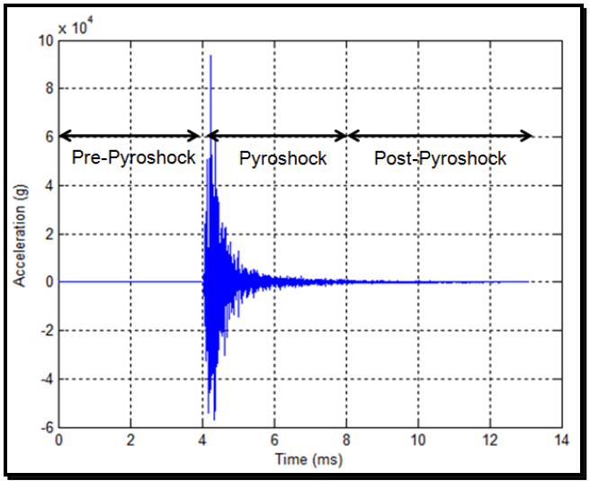
Figure description:
Acceleration vs. Time During a Pyroshock Event
Annotations
- Pre-Pyroshock (shaded_area - position: Time = 0 to 4 ms)
- Pyroshock (shaded_area - position: Time = 4 to 8 ms)
- Post-Pyroshock (shaded_area - position: Time = 8 to 13 ms)
| Time (ms) | Acceleration (g) |
|---|---|
| 0 | 0 |
| 1 | 0 |
| 2 | 0 |
| 3 | 0 |
| 4.0 | 0 |
| 4.1 | 51000 |
| 4.2 | 94000 |
| 4.3 | -57000 |
| 4.4 | 42000 |
| 4.5 | -28000 |
| 4.6 | 31000 |
| 4.8 | 21000 |
| 5.0 | 11000 |
| 5.5 | 5000 |
| 6.0 | 3000 |
| 7.0 | 1500 |
| 8.0 | 800 |
| 9.0 | 400 |
| 10.0 | 200 |
| 11.0 | 100 |
| 12.0 | 0 |
| 13.0 | 0 |
Notes: The y-axis is labeled 'Acceleration (g' with a scale factor of 10^4 at the top left. The data shows a sudden onset of high-frequency oscillations starting at 4 ms, which decay as time progresses.)
Figure 517.3-1. Full duration near-field, laser pyroshock time history (mean removed, filtered at 200 KHz).
MIL-STD-810H METHOD 517.3
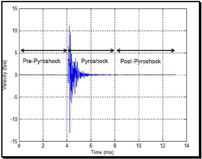
Figure description:
Pyroshock Velocity Profile
Velocity Response during Pyroshock Event
Annotations
- Pre-Pyroshock (shaded_area - position: Time = 0 to 4 ms)
- Pyroshock (shaded_area - position: Time = 4 to 8 ms)
- Post-Pyroshock (shaded_area - position: Time = 8 to 13 ms)
| Time (ms) | Velocity (fps) |
|---|---|
| 0.0 | 0.0 |
| 1.0 | 0.0 |
| 2.0 | 0.0 |
| 3.0 | 0.0 |
| 3.8 | 0.0 |
| 4.0 | 0.0 |
| 4.1 | 8.5 |
| 4.2 | -13.2 |
| 4.3 | 11.2 |
| 4.4 | -6.5 |
| 4.5 | 5.0 |
| 4.6 | -4.8 |
| 4.7 | 3.2 |
| 4.8 | -4.0 |
| 4.9 | 2.5 |
| 5.0 | -2.1 |
| 5.5 | 1.2 |
| 6.0 | -0.6 |
| 7.0 | 0.3 |
| 8.0 | 0.0 |
| 9.0 | 0.0 |
| 10.0 | 0.0 |
| 11.0 | 0.0 |
| 12.0 | 0.0 |
| 13.0 | 0.0 |
Notes: The chart shows a high-frequency oscillatory velocity response that is highly damped after the initial impact at approximately 4 ms. The regions 'Pre-Pyroshock', 'Pyroshock', and 'Post-Pyroshock' are labeled with horizontal double-headed arrows indicating time intervals.
Figure 517.3-2. Full duration near-field, laser pyroshock velocity time history.
(1) Effective Transient Duration: The "effective transient duration," Te, is defined in this Method to be the minimum length of time that contains all significant amplitude time history magnitudes beginning at the noise floor of the instrumentation system just prior to the initial most significant measurement, and proceeding to the point that the amplitude time history is a combination of measurement noise and substantially decayed structural response. In general, an experienced analyst is required to determine the pertinent measurement information to define the pyroshock event. The longer the duration of the pyroshock, the more low frequency information is preserved that may be important in far-field test considerations for the pyroshock. For near-field test considerations, in general, the effective transient duration will be much shorter because of the nature of the event. The amplitude criterion requires that the amplitude of the post-pyroshock amplitude time history envelope be no more than 12 dB above the noise floor of the measurement system depicted in the pre-pyroshock amplitude time history. From Figure 517.3-1, there is a time interval for the duration of the pyroshock based on the velocity time history in Figure 517.3-2 that clearly shows that the pyroshock event is over after 4 milliseconds. The "effective transient duration," Te, occurs from 4 milliseconds to 8 milliseconds when the velocity time history in Figure 517.3-2 effectively returns to zero. Consequently, there are 4 milliseconds of pre- pyroshock information, 4 milliseconds of pyroshock, information, and 5 milliseconds of post- pyroshock information. Figure 517.3-3 has the acceleration time history for the same event shown in Figure 517.3-1 (side-by-side measurements), and shows lower amplitudes than the laser Doppler vibrometer data in Figure 517.3-1. This will always occur because the accelerometer has a larger measurement area than the laser Doppler vibrometer that is essentially a point measurement. Thus, the accelerometer acts as a spatial integrator. The initial noise floor level is never obtained after the long duration pyroshock. Figure 517.3-4 contains the integral of Figure 517.3-3, and has the same time intervals as the laser Doppler vibrometer measurement. The magnitude of the SRS at selected natural frequencies (particularly high frequencies) can be quite insensitive to the effective transient duration. As Figure 517.3-5 demonstrates, the low frequency pyroshock SRS slope is + 9 dB/octave to + 12 dB/octave slope (or +1.5 to +2.0 on a log-log plot). The “knee" frequency is the dominant frequency in a pyroshock SRS, at which the slope for the SRS changes from an approximate + 9 dB/octave to + 12 dB/octave slope to an approximately horizontal slope with peaks at the major local structural frequencies. All pyroshock SRS have a knee frequency, even if not properly measured or
quantified. Paragraph 6.1, reference b, details the different SRS characteristics of near-field pyroshock (no "knee" frequency below 10,000 Hz) and mid-field and far-field pyroshock containing a “knee” frequency in their respective frequency ranges.
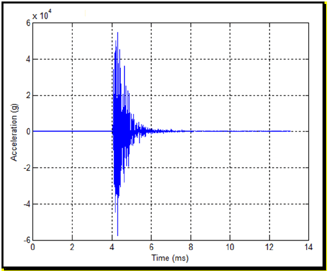
Figure description:
Acceleration vs. Time
| Time (ms) | Acceleration (g) |
|---|---|
| 0.0 | 0 |
| 1.0 | 0 |
| 2.0 | 0 |
| 3.0 | 0 |
| 3.9 | 0 |
| 4.0 | 0 |
| 4.1 | 48000 |
| 4.2 | -52000 |
| 4.3 | 55000 |
| 4.4 | -58000 |
| 4.5 | 45000 |
| 4.7 | 20000 |
| 5.0 | 10000 |
| 5.5 | 5000 |
| 6.0 | 2000 |
| 7.0 | 500 |
| 8.0 | 0 |
| 10.0 | 0 |
| 12.0 | 0 |
| 13.0 | 0 |
Notes: The y-axis values are scaled by 10^4 as indicated by the 'x 10^4' label at the top of the axis. The signal represents a high-frequency transient event starting at approximately 4 ms and decaying by approximately 8 ms.
Figure 517.3-3. Full duration near-field, accelerometer pyroshock time history.
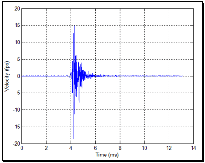
Figure description:
| Time (ms) | Velocity (fps) |
|---|---|
| 0.0 | 0.0 |
| 1.0 | 0.1 |
| 2.0 | -0.1 |
| 3.0 | 0.1 |
| 3.8 | -0.2 |
| 3.9 | 1.0 |
| 4.0 | -1.5 |
| 4.1 | 4.5 |
| 4.2 | -18.5 |
| 4.25 | 12.5 |
| 4.3 | 15.0 |
| 4.35 | -11.2 |
| 4.4 | 6.0 |
| 4.5 | -6.2 |
| 4.6 | 4.2 |
| 4.7 | -7.5 |
| 4.8 | 3.8 |
| 4.9 | -3.5 |
| 5.0 | 1.8 |
| 5.2 | 1.2 |
| 5.5 | 0.5 |
| 6.0 | 0.2 |
| 7.0 | -0.1 |
| 8.0 | 0.1 |
| 9.0 | -0.2 |
| 10.0 | 0.1 |
| 11.0 | -0.1 |
| 12.0 | 0.0 |
| 13.0 | 0.0 |
Notes: The chart shows a high-frequency velocity signal that is mostly stable near zero until approximately 4 ms, where it experiences a sharp impulsive event with peak velocities of approximately +15 fps and -18.5 fps. The signal then decays back towards zero over the next 2 ms and remains stable through 13 ms.
Figure 517.3-4. Full duration near-field, accelerometer pyroshock velocity time history.
MIL-STD-810H METHOD 517.3
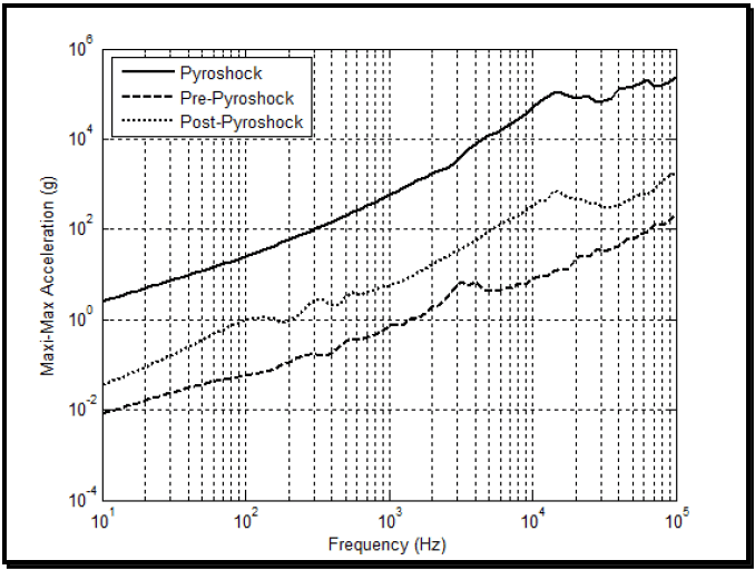
Figure description:
Legend
- Pyroshock — color: black; symbol: Solid line
- Pre-Pyroshock — color: black; symbol: Dashed line
- Post-Pyroshock — color: black; symbol: Dotted line
| Frequency (Hz) | Pyroshock (g) | Pre-Pyroshock (g) | Post-Pyroshock (g) |
|---|---|---|---|
| 10 | 2.5 | 0.008 | 0.035 |
| 20 | 5.5 | 0.015 | 0.07 |
| 50 | 18 | 0.035 | 0.25 |
| 100 | 45 | 0.06 | 0.9 |
| 200 | 95 | 0.15 | 0.9 |
| 500 | 300 | 0.4 | 4.5 |
| 1000 | 650 | 0.7 | 6.5 |
| 2000 | 2200 | 1.8 | 20 |
| 5000 | 14000 | 5 | 130 |
| 10000 | 55000 | 10 | 500 |
| 20000 | 95000 | 25 | 450 |
| 50000 | 160000 | 60 | 650 |
| 100000 | 280000 | 200 | 2000 |
Notes: The chart uses a log-log scale for both Frequency (Hz and Maxi-Max Acceleration (g. Data points are approximate values estimated from the chart's logarithmic axes.))
Figure 517.3-5. Acceleration maximax SRS for the pyroshock, pre-pyroshock and post pyroshock (laser).
(2) Shock Response Spectrum analysis: Paragraph 6.1, references e and f, defines the absolute acceleration maximax Shock Response Spectrum (SRS), and provides examples of SRS computed for classical pulses. The SRS value at a given un-damped oscillator natural frequency, f, is defined to be the absolute value of the maximum of the positive and negative acceleration responses of a mass for a given base input to a damped single degree of freedom system. The base input is the measured shock over a specified duration (the specified duration should be the effective transient duration, Te). For processing of pyroshock response data, the absolute acceleration maximax SRS has become the primary analysis descriptor. In this measurement description of the pyroshock, the maximax absolute acceleration values are plotted on the ordinate with the un-damped natural frequency of the single degree of freedom system, with base input plotted along the abscissa. A more complete description of the pyroshock (and potentially more useful for pyroshock damage comparison in the far-field) can be obtained by determining the maximax pseudo-velocity response spectrum and plotting this on four- coordinate paper where, in pairs of orthogonal axes, (1) the maximax pseudo-velocity response spectrum is represented by the ordinate with the un-damped natural frequency being the abscissa, and (2) the maximax absolute acceleration along with the maximax pseudo-displacement plotted in a pair of orthogonal axes (paragraph 6.1, reference e). The maximax pseudo-velocity at a particular oscillator un-damped natural frequency is thought to be more representative of the damage potential for a shock since it correlates with stress and strain in the elements of a single degree of freedom system (paragraph 6.1, references f, g, and h). The maximax pseudo-velocity response spectrum can be computed either by (1) dividing the maximax absolute acceleration response spectrum by the un- damped natural frequency of the single degree of freedom system, or (2) multiplying the maximax relative displacement by the un-damped natural frequency of the single degree of freedom system. Both means of computation provide essentially the same spectra except possibly in the lower frequency region, in which case the second method of computation is more basic to the definition of the maximax pseudo-velocity response spectrum. Figure 517.3-5 provides the maximax absolute acceleration SRS for the pyroshock record on Figure 517.3-1. Figure 517.3-6 provides the maximax pseudo-velocity for this record on four-coordinate paper. Information below 100 Hz for the maximax acceleration SRS may reveal data anomalies not detected otherwise or confirm erroneous velocity change (see Annex A of this Method). Figure 517.3-6 shows that maximum pseudo-velocity of almost
500 ips occurs above 10,000 Hz. The high velocity change at high frequency is indicative of the damage potential for electronic components. In general, compute the SRS over the pyroshock event duration and over the same duration for the pre-pyroshock and the post-pyroshock events with twelfth octave spacing, and a Q = 10 (Q=10 corresponds to a single degree of freedom system with 5 percent critical damping). If the testing is to be used for laboratory simulation, use a second Q value of 50 (Q=50 corresponds to a single degree of freedom system with 1 percent critical damping) in the processing. It is recommended that the maximax absolute acceleration SRS be the primary method of display for the pyroshock and the maximax pseudo-velocity SRS be the secondary method of display. The maximax pseudo-velocity SRS is useful in cases in which it is desirable to correlate damage of simple systems with the pyroshock.
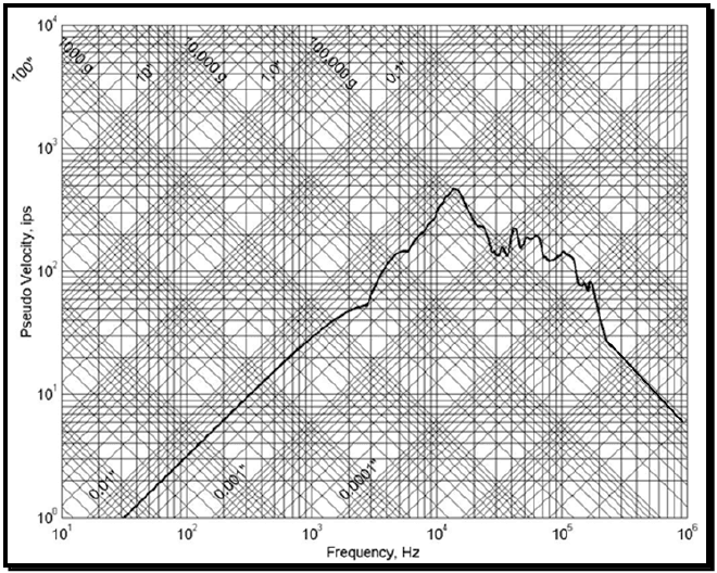
Figure description:
Annotations
- 100" (text_label - position: Constant displacement diagonal line (slope +1))
- 10" (text_label - position: Constant displacement diagonal line (slope +1))
- 1.0" (text_label - position: Constant displacement diagonal line (slope +1))
- 0.1" (text_label - position: Constant displacement diagonal line (slope +1))
- 0.01" (text_label - position: Constant displacement diagonal line (slope +1))
- 0.001" (text_label - position: Constant displacement diagonal line (slope +1))
- 0.0001" (text_label - position: Constant displacement diagonal line (slope +1))
- 1000 g (text_label - position: Constant acceleration diagonal line (slope -1))
- 10,000 g (text_label - position: Constant acceleration diagonal line (slope -1))
- 100,000 g (text_label - position: Constant acceleration diagonal line (slope -1))
| Frequency (Hz) | Pseudo Velocity (ips) |
|---|---|
| 20 | 0.6 |
| 30 | 1.0 |
| 50 | 1.6 |
| 100 | 3.3 |
| 200 | 6.5 |
| 300 | 10.0 |
| 500 | 16.0 |
| 1000 | 33.0 |
| 2000 | 50.0 |
| 3000 | 55.0 |
| 4000 | 105.0 |
| 5000 | 130.0 |
| 8000 | 180.0 |
| 10000 | 250.0 |
| 13000 | 440.0 |
| 15000 | 370.0 |
| 20000 | 250.0 |
| 25000 | 180.0 |
| 28000 | 140.0 |
| 30000 | 160.0 |
| 32000 | 140.0 |
| 35000 | 140.0 |
| 41000 | 210.0 |
| 44000 | 160.0 |
| 52000 | 195.0 |
| 57000 | 180.0 |
| 62000 | 205.0 |
| 80000 | 120.0 |
| 100000 | 155.0 |
| 120000 | 130.0 |
| 150000 | 80.0 |
| 160000 | 90.0 |
| 200000 | 35.0 |
| 400000 | 15.0 |
| 700000 | 8.0 |
| 1000000 | 6.0 |
Notes: The chart is a Tripartite Log-Log plot typical for Shock Response Spectra (SRS. The primary axes are Frequency (Hz and Pseudo Velocity (ips. Diagonal grid lines provide reference for constant displacement (inches and constant acceleration (g.)))))
Figure 517.3-6. Maximax pseudo-velocity response spectrum for the pyroshock (laser).
- (3) Other Methods: Over the past few years, at least two other techniques potentially useful in processing pyroshock data have been suggested. Paragraph 6.1, reference i, describes the use of time domain or temporal moments for comparing the characteristics of the pyroshock over different frequency bands. The usefulness of this technique resides in the fact that if the pyroshock can be represented by a simple non-stationary product model, the time domain moments must be constant over selected filter bandwidths. Thus, the pyroshock can be characterized by a model with potential usefulness for stochastic simulation. Paragraph 6.1, reference j, explores this reasoning for mechanical shock. Paragraph 6.1, reference k, describes the use of wavelets for vibration. It has been suggested that wavelet processing may be useful for pyroshock description, particularly if a pyroshock contains information at intervals of time over the duration of the shock at different time scales, i.e., different frequencies.
- b. In general, for pyroshock tests, a single response record is obtained. At times, it may be convenient or even necessary to combine equivalent processed responses in some appropriate statistical manner. Paragraph 6.1, references a and 1, and Method 516.8, Annex B of this Standard discuss some options in statistically summarizing processed results from a series of tests. In general, processed results, either from the SRS, ESD, or FS are logarithmically transformed in order to provide estimates that are more normally distributed. This
is important since often very little data are available from a test series, and the probability distribution of the untransformed estimates cannot be assumed to be normally distributed. In general, the combination of processed results will fall under the category of small sample statistics and needs to be considered with care. Parametric or less powerful nonparametric methods of statistical analysis may usually be effectively applied.
2.3.2 Single Pyroshock Event Measurement System Characterization and Basic Processing
The following paragraphs discuss basic measurement system acquisition characteristics, followed by a discussion of the correct identification of the parts of a measured pyroshock (in particular the duration of a pyroshock). Information in Method 516.8, Annex A and Annex A of this Method is essential for the processing of measured data for a laboratory test specification.
In this paragraph with its subdivisions, proper identification of a single pyroshock will be illustrated. Once the pyroshock has been correctly identified, processing is generally routine as per the details in paragraph 2.3.1. Pyroshock event identification is important for deciding upon the manner of testing in the laboratory. Within the time domain characterization, anticipating further digital processing, it is assumed the measured data are properly signal conditioned, and subsequently digitized with a minimum of aliased information into the bandwidth of interest (less than five percent) and, in general, the measurement time history has been validated. Details for validation are contained Paragraph 6.1, references b and d.
The following information corresponding to the time domain characterization must be present for assessment by an analyst in establishing pyroshock requirements:
- a. Signal bandwidth, i.e., DC to where is the maximum frequency of interest consistent with the analog, anti-alias filter design built into the analog signal conditioning , i.e., where is the 3dB half-power point cut-off frequency of the lowpass analog anti-alias filter. Generally, for SRS analysis in order to get accurate estimates at , it is required that the analog, anti-alias rolloff be taken into account so that it does not interfere with the SRS filter estimates at . Likewise, digital filters must be in place before digital decimation.
- b. Digital signal sample rate Fs, shall be such that the anti-alias filter provides a minimum attenuation as shown in Figure 517.3-7. The digitizing rate shall be at least 1 MHz or higher as per Paragraph 6.1, reference p. Paragraph 6.1, references b and d, recommend a minimum 60 dB/octave anti-alias filter, with the half-power point cut-off frequency set at fc < 0.6* fNyquist. The requirements of this section are an equivalent way to achieve the same aliasing protection with more flexibility in other data parameters. For higher rates of roll- off, fc can be increased, but must never exceed 0.8* fNyquist. For 10* fmax < Fs, re-sampling will be necessary for SRS computation to preserve filtering accuracy. The final sample rate shall meet or exceed ten times the maximum frequency of interest, i.e., Fs > 10* fmax.
- c. The data recording instrumentation shall have flat frequency response to at least 100 kHz for all channels at each measurement location. Attenuation of 3 dB at 100 kHz is acceptable. The digitizing rate must be at least 1 MHz or higher so that measurements of peak amplitude to qualify the shock level are accurate. Additional, lower frequency measurement channels, at the same location may be used for lower frequency response measurements.
It is imperative that a responsibly designed system to reject aliasing is employed. Analog anti-alias filters must be in place before the digitizer. The selected anti-alias filtering must have an attenuation of 50 dB or greater, and a pass band flatness within +/- 1.0 dB and phase linearity to within +/- 5° across the frequency bandwidth of interest for the measurement (see Figure 517.3-7). Subsequent resampling e.g., for purposes of decimation, must be in accordance with standard practices and consistent with the analog anti-alias configuration (e.g. digital filters must be in place before subsequent decimations).
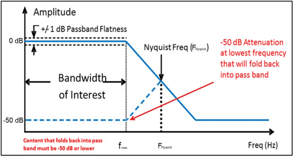
Figure description:
System Frequency Response Filter and Aliasing Performance Requirements
Amplitude vs Frequency Response
Legend
- Amplitude Response — color: blue; symbol: solid line
- Aliased Signal Content — color: blue; symbol: dashed line
- Passband and Attenuation Limits — color: black/blue; symbol: dashed lines
Annotations
- +/- 1 dB Passband Flatness (text_label - position: y = 0, frequency 0 to f_max)
- Bandwidth of Interest (horizontal_range - position: x-axis from 0 to f_max)
- Nyquist Freq (F_Nyquist (vertical_line - position: x = F_Nyquist))
- -50 dB Attenuation at lowest frequency that will fold back into pass band (text_label - position: Red arrow pointing from (2 * F_Nyquist - f_max, -50 to (f_max, -50)))
- Content that folds back into pass band must be -50 dB or lower (text_label - position: Bottom left, below the frequency axis)
| Frequency | Amplitude (solid blue (dB)) | Aliased Content (dashed blue (dB)) | Upper Passband Flatness (dB) | Lower Passband Flatness (dB) | Foldback Limit (dB) |
|---|---|---|---|---|---|
| 0 | 0 | -50 | 1 | -1 | -50 |
| f_max | 0 | -50 | 1 | -1 | -50 |
| F_Nyquist | -25 | -25 | null | null | null |
| 2 * F_Nyquist - f_max | -50 | null | null | null | null |
| Frequency Max | -50 | null | null | null | null |
Notes: The graph illustrates filter requirements to prevent aliasing. It shows the main signal amplitude roll-off and the mirrored 'aliased' signal folding back from the Nyquist frequency. The requirements specify a +/- 1 dB passband flatness within the bandwidth of interest (up to f_max and a minimum of 50 dB attenuation for any content folding back into this band.)
Figure 517.3-7. Filter attenuation (conceptual, not filter specific).
The end to end alias rejection of the final digitized output must be shown to meet the requirements in Figure 517.3-7. The anti-alias characteristics must provide an attenuation of 50 dB or greater for frequencies that will fold back into the passband. Spectral data including SRS plots may only be presented for frequencies within the passband (between 0 and ). However, this restriction is not to constrain digital data validation procedures that require assessment of digitally acquired data to the Nyquist frequency (either for the initial ADC or subsequent resampled sequences). It should be noted that it is possible that certain sensor/signal conditioning systems may display substantial “out-of-band” frequency content, i.e., greater than but less than the Nyquist frequency, in digital processing. For example, a Fourier spectra estimate over the duration of the shock may display “general signal” to “noise” that seemingly contradicts the filter attenuation criterion displayed in Figure 517.3-7. In this case the signal conditioning/digitizing system must be subject to the “verification of alias rejection” described in the paragraph to follow. If the signal conditioning system is verified as non-aliasing then the substantial frequency content between and the Nyquist frequency can be digitally filtered out if desired.
Verification of alias rejection should start by establishing the dynamic range within the pass band in terms of the signal to noise ratio (SNR). The voltage-based SNR = 20log ( 10 V FullScale V Noisefloor ) must be ≥60dB. Once sufficient SNR is verified, establishing the alias rejection characteristics may be determined using an input sine wave with a magnitude of 0.5 * full scale range and at the lowest frequency range that can impinge i.e., be aliased into 𝑓𝑓𝑀𝑀𝑀𝑀𝑀𝑀, and then confirming (using the IEEE 1057 sine wave test procedure or through inspection of the time domain data) that the alias rejection is sufficient at this frequency for the signal conditioning system.
For a conventional multi-bit ADC such as flash or successive approximation design, if a 1 million sample/second digitizing rate is used, for example, then 𝑓𝑓𝑁𝑁𝑁𝑁𝑁𝑁𝑁𝑁𝑁𝑁𝑁𝑁𝑁𝑁= 500 KHz. Theory says that if a signal above the Nyquist Ratio is present, it will “fold over” into a frequency below the Nyquist ratio. The equation is:
Fa = absolute value [(Fs*n)-F], where
of "alias"
F = frequency of input signal
Fs = sample rate
n = integer number of sample rate (Fs) closest to input signal frequency (F)
Hence, the lowest frequency range that can fold back into the 100 KHz passband is from 900 KHz to 1.1 MHz.
It should be noted that Sigma Delta (SD) digitizers “oversample” internally at a rate several times faster than the output data rate and that analog anti-alias filtering is still required. For illustrative purposes, consider an example for a SD digitizer with a bandwidth of interest up to 100 KHz that samples internally at million samples/second. The internal analog based Nyquist frequency by definition is 4 MHz, hence the analog anti-alias filter should attenuate 50 dB or more content that can fold back into the 100 KHz pass band (7.9 MHz to 8.1 MHz and similar bands that are higher in frequency). Figure 517.3.8 illustrates sampling frequencies, Nyquist frequencies, and frequency bands that can fold back into the bandwidth of interest for both conventional and over sampling digitizers, such as the Sigma Delta. Observe that for the example SD design, there is significant bandwidth above the 100 KHz desired and the Nyquist rate that is not useable due primarily to quantization error, an artifact of the single bit SD design. The output of a SD ADC will be digitally filtered and resampled yielding a new effective sampling rate which in turn yields a new Nyquist rate for the decimated signal of . Through careful selection the digital filter cutoff frequency, the majority of noise between and is removed while maintaining a nearly flat frequency response through . The SD oversampling rate , which is directly correlated to dynamic range, is one of several design parameters for a SD ADC. Most reputable vendors will provide a detailed specification sheet associated with their products, however, it is strongly recommended that one verifies aliasing rejection and noise floor characteristics as recommended above prior to employing any signal conditioning/digitizing system in the acquisition of critical field data.
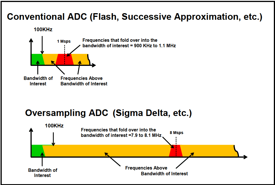
Figure description:
Comparison of Conventional vs. Oversampling ADC Aliasing
Conventional ADC (Flash, Successive Approximation, etc.
Legend
- Bandwidth of Interest — color: Green; symbol: Solid region
- Frequencies Above Bandwidth of Interest — color: Orange; symbol: Solid region
- Frequencies that fold over into the bandwidth of interest — color: Red; symbol: Solid region
- Sampling Rate — color: Black; symbol: Dashed vertical line
Annotations
- 100KHz (text_label - position: x = 100 KHz)
- 1 Msps (vertical_line - position: x = 1 Msps)
- Frequencies that fold over into the bandwidth of interest = 900 KHz to 1.1 MHz (text_label - position: Centered over the red region at 1 MHz)
| Segment | Frequency Range | Color |
|---|---|---|
| Bandwidth of Interest | 0 - 100 KHz | Green |
| Frequencies Above Bandwidth of Interest (part 1) | 100 KHz - 900 KHz | Orange |
| Frequencies that fold over into the bandwidth of interest | 900 KHz - 1.1 MHz | Red |
| Frequencies Above Bandwidth of Interest (part 2) | > 1.1 MHz | Orange |
Oversampling ADC (Sigma Delta, etc.
Legend
- Bandwidth of Interest — color: Green; symbol: Solid region
- Frequencies Above Bandwidth of Interest — color: Orange; symbol: Solid region
- Frequencies that fold over into the bandwidth of interest — color: Red; symbol: Solid region
- Sampling Rate — color: Black; symbol: Dashed vertical line
Annotations
- 100KHz (text_label - position: x = 100 KHz)
- 8 Msps (vertical_line - position: x = 8 Msps)
- Frequencies that fold over into the bandwidth of interest = 7.9 to 8.1 MHz (text_label - position: Centered over the red region at 8 MHz)
| Segment | Frequency Range | Color |
|---|---|---|
| Bandwidth of Interest | 0 - 100 KHz | Green |
| Frequencies Above Bandwidth of Interest (part 1) | 100 KHz - 7.9 MHz | Orange |
| Frequencies that fold over into the bandwidth of interest | 7.9 - 8.1 MHz | Red |
| Frequencies Above Bandwidth of Interest (part 2) | > 8.1 MHz | Orange |
Notes: The diagrams illustrate how increasing the sampling rate (oversampling moves the aliasing frequencies (the red region that 'folds over' into the bandwidth of interest further away from the desired signal bandwidth (0 to 100 KHz.)))
Figure 517.3-8. Illustration of sampling rates and out of band "fold over" frequencies for Conventional and Oversampling (Sigma-Delta) based data acquisition systems.
- d. A noise gage is required for pyroshock measurements because it assists in the identification of anomalies in the data. The noise gage, or inert accelerometer may be purchased from most accelerometer manufacturers. Additionally, the noise gage may also be the same transducer as for other measurement channels and simply suspended near, but not on, the materiel.
2.3.3 Test Conditions – Shock Spectrum Transient Duration and Scaling
Derive the SRS and the effective transient duration, Te, from measurements of the materiel's environment or, if available, from dynamically scaled measurements of a similar environment. Because of the inherent high degree of measurement randomness and limited response prediction methodology associated with the response to a pyroshock, extreme care must be exercised in dynamically scaling a similar event. For pyroshocks, there are two known scaling laws for use with response from pyroshocks that may be helpful if used with care (paragraph 6.1, reference a).
2.3.3.1 Pyroshock Source Energy Scaling (SES)
The first scaling law is the Source Energy Scaling (SES) where the SRS is scaled at all frequencies by the ratio of the total energy release of two different devices. For (reference energy) and (new energy), the total energy in two pyrotechnic shock devices, the relationship between the SRS processed levels at a given natural frequency and distance is given by the following expression:
In using this relationship, it is assumed that either an increase or decrease in the total energy of the pyrotechnic shock devices will be coupled into the structure in exactly the same way, i.e., excessive energy from a device will go into the structure, as opposed to being dissipated in some other way, e.g., through the air. En and Er may come from physical considerations related to the pyrotechnic device or be computed from ESD estimates (or in the time domain by way of a Parseval-form relationship) where it is assumed that the time history measurements quantify the energy difference. Paragraph 6.1, reference a, discusses conditions under which this scaling law may lead to over-prediction for En > E, or under-prediction when E <E.
2.3.3.2 Pyroshock Response Location Distance Scaling (RLDS)
The second scaling law is the Response Location Distance Scaling (RLDS) where the SRS is scaled at all frequencies by an empirically derived function of the distance between two sources. For D1 and D2, the distances (in meters) from a pyrotechnic shock device (point source), the relationship between the SRS processed levels at a given natural frequency, fn, is given by the following expression:
SRS(D2) = SRS(D₁)exp {|- 8×10⁴ f -4 (2.4fn -0.105) (D₂-D1)} 2-D.
In using this relationship, it is assumed that D1 and D2 can be easily defined as in the case of a pyrotechnic point source device. Figure 517.3-9 from paragraph 6.1, reference a, displays the ratio of SRS(fn|D2) to SRS(fn|D1) as a function of the natural frequency, fn, for selected values of D2-D1. It is clear from this plot that, as the single degree of freedom natural frequency increases, there is a marked decrease in the ratio for a fixed D2-D1 > 0 and as D2-D1 increases the attenuation becomes substantial. This scaling relationship when used for prediction between two configurations relies very heavily upon (1) similarity of configuration, and (2) the same type of pyrotechnic device. Consult paragraph 6.1, reference a, before applying this scaling relationship.
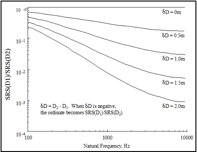
Figure description:
SRS Ratio as a Function of Natural Frequency and Distance Difference
SRS(D1/SRS(D2 vs Natural Frequency
Legend
- δD = 0m — color: black; symbol: Solid line
- δD = 0.5m — color: black; symbol: Solid line
- δD = 1.0m — color: black; symbol: Solid line
- δD = 1.5m — color: black; symbol: Solid line
- δD = 2.0m — color: black; symbol: Solid line
Annotations
- δD = D2 - D1. When δD is negative, the ordinate becomes SRS(D2/SRS(D1. (text_label - position: Centered in the lower-left quadrant of the plot area)))
| Natural Frequency (Hz) | δD = 0m | δD = 0.5m | δD = 1.0m | δD = 1.5m | δD = 2.0m |
|---|---|---|---|---|---|
| 100 | 1.0 | 0.80 | 0.60 | 0.40 | 0.30 |
| 200 | 1.0 | 0.68 | 0.42 | 0.24 | 0.14 |
| 500 | 1.0 | 0.48 | 0.20 | 0.075 | 0.030 |
| 1000 | 1.0 | 0.38 | 0.12 | 0.030 | 0.010 |
| 2000 | 1.0 | 0.30 | 0.075 | 0.014 | 0.0035 |
| 5000 | 1.0 | 0.24 | 0.045 | 0.0080 | 0.0015 |
| 10000 | 1.0 | 0.22 | 0.038 | 0.0065 | 0.0011 |
Notes: The chart is presented on a log-log scale. The Y-axis represents the ratio SRS(D1/SRS(D2 from 10^-4 to 10^0. The X-axis represents Natural Frequency in Hz from 100 to 10,000.))
Figure 517.3-9. Empirical scaling relationship for shock response spectrum as a function of the distance from the pyrotechnic source.
2.3.3.3 Measured Data Available From Pyroshock
- a. If measured acceleration data are available, the acceleration data shall be validated prior to use. The best indicator of the acceleration data quality is its integral or velocity time history as in paragraph 6.1, references b and d, that shall reflect the physical test configuration that is, in general, zero before and after a pyroshock test. Anomalies in the velocity time history shall be investigated as per paragraph 6.1, references b and d, and their source documented. If the requirements of Paragraph 2.3.2 of this document, were not used to prevent aliasing contamination of the data, then exceptions to these criteria shall be documented and sufficiently justified to prove that digital aliasing of the data has not occurred. Additionally, if all components in the data acquisition system do not have linear phase-shift characteristics in the data passband, and do not have a passband uniform to within one dB across the frequency band of interest, exceptions to these criteria shall be documented and sufficiently justified to prove that data contamination have not occurred.
- b. If measured data are available, the data may be processed using the SRS, FS, or ESD. For engineering and historical purposes, the SRS has become the standard for measured data processing. In the discussion to follow, it will be assumed that the SRS is the processing tool. In general, the maximax SRS spectrum (absolute acceleration or absolute pseudo-velocity) is the main quantity of interest. With this background, determine the shock response spectrum required for the test from analysis of the measured environmental acceleration time history. After carefully qualifying the data, to make certain there are no anomalies in the amplitude time history, according to the recommendations provided in paragraph 6.1, references b and d, compute the SRS. The analysis will be performed for Q = 10 at a sequence of natural frequencies at intervals of at least 1/6 octave, and no finer than 1/12th octave spacing to span at least 100 to 20,000 Hz, but not to exceed 100,000 Hz. The frequency range over which the SRS is computed, (i.e., natural frequencies of the SDOF system filters) as a minimum, includes the data signal conditioning bandwidth, but should also extend below and above this bandwidth. In general, the “SRS Natural Frequency Bandwidth” extends from an octave below the lowest frequency of interest, up to a frequency at which the “flat” portion of the SRS spectrum has been reached (that may require going an octave or more above the upper signal conditioning bandwidth). This latter SRS upper frequency, , requirement helps ensure no high frequency content in the spectrum is neglected, and is independent of the data bandwidth upper frequency, . As a minimum, this SRS upper frequency should exceed by at least ten percent, i.e., . The lowest frequency of interest is determined by the frequency response characteristics of the mounted materiel under test. Define as the first mounted natural frequency of the materiel (by definition, will be less than or equal to the first
natural frequency of a materiel component such as a circuit board) and, for laboratory testing purposes, define the lowest frequency of interest as ( i.e., is at least one octave below ). can then be taken as . The maximax SRS is to be computed over the long time duration and over the frequency range from to . When a sufficient number of representative shock spectra are available, employ an appropriate statistical technique (an enveloping technique) to determine the required test spectrum. Annex B of Method 516.8 references the appropriate statistical techniques. Parametric statistics can be employed if the data can be shown to satisfactorily fit an assumed underlying probability distribution. When a normal or lognormal distribution can be justified, Annex B of Method 516.8, and paragraph 6.1, reference 1 of this Method, references a and 1, provide a method for estimating such a test level. Test levels based upon a maximum predicted environment defined to be equal to or greater than the 95th percentile value at least 50 percent of the time uses a one-sided tolerance interval approach.
- c. When insufficient data are available for statistical analysis, use an increase over the maximum of the available spectral data to establish the required test spectrum to account for randomness and inherent variability of the environment. The degree of increase is based upon engineering judgment and is supported by rationale for that judgment. In these cases, it is often convenient to envelope the SRS by computing the maximax spectra over the sample spectra, and proceed to add a +6dB margin to the SRS maximax envelope over the entire frequency range of interest.
- d. When employing the pyroshock method, determine the effective transient duration, Te, from the measurement time histories of the environmental data as suggested in paragraph 2.3.1. For all procedures, the pyroshock amplitude time history used for the SRS analysis will be Te in duration. In addition, measurement data for a duration, Te, shall be collected just prior to the pyroshock, and duration, Te, just after the pyroshock for subsequent analysis. In general, each individual axis of the three orthogonal axes will have approximately the same shock test SRS and average effective duration as a result of the omni-directional properties of a pyroshock in Procedure I and Procedure II. For Procedures III, IV, and V, the form of shock test SRS may vary with axes. Use an SRS shaker shock replication method when using Procedure V; do not use classical shock pulse forms, e.g., half-sine, terminal-peak saw tooth, etc., in the testing.
2.3.3.4 Measured Data Not Available From Pyroshock
If a database is not available for a particular configuration, use configuration similarity and any associated measured data for prescribing a pyroshock. Because of the sensitivity of the pyroshock to the system configuration and the wide randomness and variability inherent in pyrotechnic measurements, the tester must proceed with caution. As a basic guide for pyroshock testing, Figure 517.3-10 from paragraph 6.1, reference m, provides SRS estimates for four typical aerospace application pyrotechnic point source devices. Figure 517.3-11 from paragraph 6.1, reference a, provides information on the attenuation of the peaks in the SRS, and of the ramp in the SRS of the point sources on Figure 517.3-10 with distance from the source. Information on Figures 517.3-10 and 517.3-11 come from paragraph 6.1, reference n. This reference also recommends the attenuation of the peak SRS across joints be taken to be 40 percent per joint for up to three joints, and that there be no attenuation of the ramp portion (portion linearly increasing with frequency on the log log plot) of the SRS. Figure 517.3-12 provides the degree of attenuation of the peak amplitude time history response as a function of the shock path distance from the source for seven aerospace structural configurations. This information was summarized from paragraph 6.1, reference o. Either the SES scaling law or the RLDS scaling law may provide guidance. In most cases, either Procedure II or Procedure III are the optimum procedures for testing, with the smallest risk of either substantial undertest or gross overtest, when Procedure I is not an option. Proceed with caution with Procedure II, Procedure III, or Procedure IV, cognizant of the information contained in paragraph 6.1, reference b. Generally, a test transient is deemed suitable if it’s SRS equals or exceeds the given SRS requirement over the minimum frequency range of 100 to 20,000 Hz, and the effective transient duration (T) of the test transient is within 20 percent of that of the normal pyroshock response transient duration (Te). (See paragraph 4.2.2 for test tolerances.)
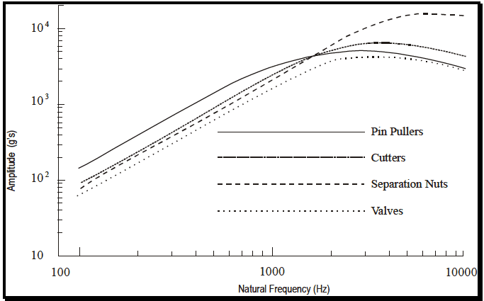
Figure description:
Shock Spectra Comparison
Amplitude vs. Natural Frequency for Pyrotechnic Shock Sources
Legend
- Pin Pullers — color: black; symbol: Solid line
- Cutters — color: black; symbol: Dash-dot line
- Separation Nuts — color: black; symbol: Dashed line
- Valves — color: black; symbol: Dotted line
| Natural Frequency (Hz) | Pin Pullers Amplitude (g's) | Cutters Amplitude (g's) | Separation Nuts Amplitude (g's) | Valves Amplitude (g's) |
|---|---|---|---|---|
| 120 | 140 | 95 | 85 | 65 |
| 200 | 250 | 180 | 160 | 120 |
| 500 | 800 | 600 | 550 | 400 |
| 1000 | 2500 | 1800 | 1500 | 1100 |
| 2000 | 4500 | 4500 | 4500 | 3000 |
| 3000 | 5000 | 5600 | 8500 | 3800 |
| 4000 | 4800 | 6200 | 12000 | 4000 |
| 6000 | 4000 | 5800 | 18000 | 3800 |
| 8000 | 3400 | 5000 | 17500 | 3200 |
| 10000 | 2800 | 4000 | 16000 | 2800 |
Notes: The chart is a log-log plot showing shock response spectra for various components. The Y-axis represents Amplitude in g's and the X-axis represents Natural Frequency in Hz.
Figure 517.3-10. Shock response spectra for various point source pyrotechnic devices.
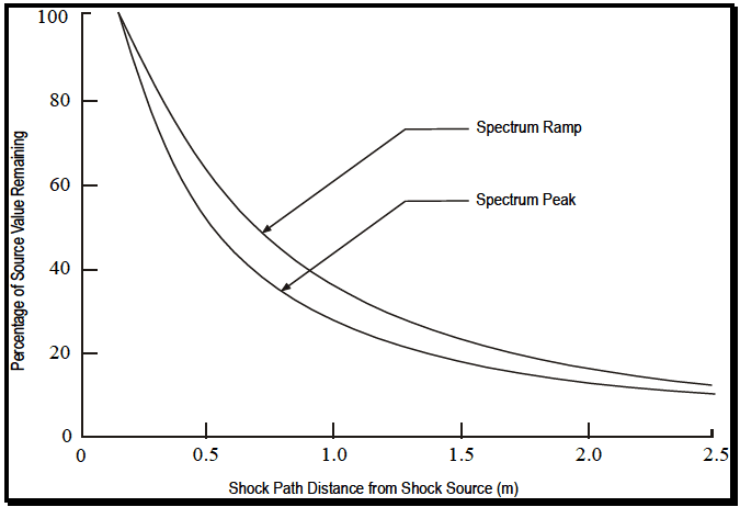
Figure description:
Legend
- Spectrum Ramp — color: black; symbol: Solid line
- Spectrum Peak — color: black; symbol: Solid line
Annotations
- Spectrum Ramp (text_label - position: Arrow pointing to the upper curve at approximately (0.8, 48))
- Spectrum Peak (text_label - position: Arrow pointing to the lower curve at approximately (0.9, 32))
| Shock Path Distance from Shock Source (m) | Spectrum Ramp (%) | Spectrum Peak (%) |
|---|---|---|
| 0.15 | 100 | 100 |
| 0.25 | 88 | 80 |
| 0.50 | 65 | 53 |
| 0.75 | 49 | 39 |
| 1.00 | 38 | 29 |
| 1.25 | 30 | 23 |
| 1.50 | 25 | 18 |
| 1.75 | 20 | 15 |
| 2.00 | 17 | 13 |
| 2.25 | 14 | 11 |
| 2.50 | 12 | 10 |
Notes: The graph depicts the decay of source value percentage over shock path distance. Both curves (Spectrum Ramp and Spectrum Peak originate at 100% at a distance of approximately 0.15 meters from the source.)
Figure 517.3-11. Shock response spectrum versus distance from pyrotechnic source.
MIL-STD-810H
METHOD 517.3
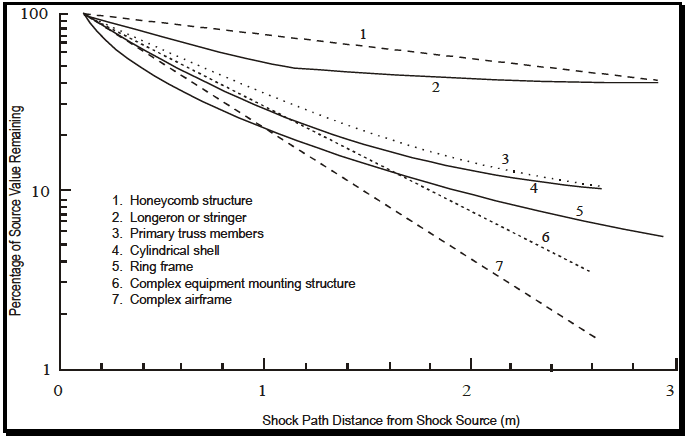
Figure description:
Shock Attenuation in Various Structural Configurations
Percentage of Source Value Remaining vs. Shock Path Distance
Legend
- 1. Honeycomb structure — color: black; symbol: Dashed line
- 2. Longeron or stringer — color: black; symbol: Solid line
- 3. Primary truss members — color: black; symbol: Dotted line
- 4. Cylindrical shell — color: black; symbol: Solid line
- 5. Ring frame — color: black; symbol: Solid line
- 6. Complex equipment mounting structure — color: black; symbol: Dotted line
- 7. Complex airframe — color: black; symbol: Dashed line
Annotations
- 1 (text_label - position: Near the end of line 1)
- 2 (text_label - position: Near the end of line 2)
- 3 (text_label - position: Near the end of line 3)
- 4 (text_label - position: Near the end of line 4)
- 5 (text_label - position: Near the end of line 5)
- 6 (text_label - position: Near the end of line 6)
- 7 (text_label - position: Near the end of line 7)
| Shock Path Distance from Shock Source (m) | 1. Honeycomb structure | 2. Longeron or stringer | 3. Primary truss members | 4. Cylindrical shell | 5. Ring frame | 6. Complex equipment mounting structure | 7. Complex airframe |
|---|---|---|---|---|---|---|---|
| 0.0 | 100.0 | 100.0 | 100.0 | 100.0 | 100.0 | 100.0 | 100.0 |
| 0.5 | 86.0 | 68.0 | 56.0 | 48.0 | 42.0 | 35.0 | 28.0 |
| 1.0 | 74.0 | 50.0 | 30.0 | 26.0 | 21.0 | 18.0 | 13.0 |
| 1.5 | 64.0 | 47.0 | 19.0 | 17.0 | 14.0 | 10.0 | 6.5 |
| 2.0 | 55.0 | 45.0 | 13.0 | 12.0 | 10.0 | 6.2 | 3.2 |
| 2.5 | 47.0 | 44.0 | 10.5 | 10.2 | 7.5 | 3.8 | 1.8 |
| 3.0 | 41.0 | 43.0 | null | null | 6.0 | null | null |
Notes: The Y-axis is on a logarithmic scale (1, 10, 100. The chart shows the attenuation of shock value across various aircraft-related structures as distance from the shock source increases.)
Figure 517.3-12. Peak pyroshock response versus distance from pyrotechnic source.
2.3.4 Test Axes, Duration, and Number of Shock Events
2.3.4.1 General
A suitable test shock for each axis is one that yields an SRS that equals or exceeds the required test SRS over the specified frequency range when using a specified duration for the test shock time history, and when the effective transient duration of the shock (Te) is within twenty percent of the specified Te value. For Procedure I, Te is not specified, but is measured. Properly validate the test data and determine the maximax acceleration SRS for Q = 10, and at least at 1/12-octave frequency intervals. The best indicator of the acceleration data quality is its integral or velocity time history as in paragraph 6.1, references b and d, that shall reflect the physical test configuration that is, in general, zero before and after a pyroshock test. Anomalies in the velocity time history shall be investigated as per paragraph 6.1, references b and d, and their source(s) documented. If the requirements of Paragraph 2.3.2 of this document, i.e. an anti-aliasing filter with attenuation as shown in Figure 517.3-7.were not used to prevent aliasing contamination of the data, then exceptions to these criteria shall be documented and sufficiently justified to prove that digital aliasing of the data has not occurred. Additionally, all components in the data acquisition system shall have linear phase-shift characteristics in the data passband, and shall have a passband uniform to within one dB across the frequency band of interest. The following guidelines may also be applied. For materiel that is likely to be exposed once to a given pyroshock event, perform one shock for each appropriate environmental condition. For materiel that is likely to be exposed more frequently to pyroshock events and there are little available data to substantiate the number of pyroshocks, apply three or more at each environmental condition based on the anticipated service use. Application of three or more shocks in one configuration is for enhancement of statistical confidence.
There is a general convention in the evaluation of the pyroshock specifications that a specification with a velocity change of 50 ips or less is mild enough that testing is not required. However, specific programs may require testing for specifications of 50 ips or less if there are components that may be sensitive to even these low velocity changes.
2.3.4.2 Procedure I - Near-field with an Actual Configuration
For Procedure I, subject the test item to a sufficient number of suitable shocks to meet the specified test conditions or at least three shocks. The objective of the test is to test the physical and functional integrity of the materiel under pyroshock in the near-field of the pyrotechnic device.
2.3.4.3 Procedure II - Near-field with a Simulated Configuration
For Procedure II, subject the test item to a sufficient number of suitable shocks to meet the specified test conditions or at least three shocks. The measured response test requirements may be satisfied along more than one axis with a single test shock configuration. Consequently, it is conceivable that a minimum of one test shock will satisfy the requirements for all directions of all three orthogonal axes. At the other extreme, a total of three shocks are required
if each shock only satisfies the test requirements in one direction of one axis. The objective of the test is to test the structural and functional integrity of the materiel under pyroshock in the near-field of the pyrotechnic device.
2.3.4.4 Procedure III - Mid-field with a Mechanical Test Device
For Procedure III, subject the test item to a sufficient number of suitable shocks to meet the specified test conditions, or at least three shocks. The measured response test requirements may be satisfied along more than one axis with a single test shock configuration. Consequently, it is conceivable that a minimum of three test shock repetitions will satisfy the requirements for all directions of all three orthogonal axes. At the other extreme, a total of nine shocks are required if each shock only satisfies the test requirements in one direction of one axis. The objective of the test is to test the structural and functional integrity of the system under pyroshock in the mid-field of the pyrotechnic device.
2.3.4.5 Procedure IV - Far-field with a Mechanical Test Device
For Procedure IV, subject the test item to a sufficient number of suitable shocks to meet the specified test conditions or at least three shocks. The measured response test requirements may be satisfied along more than one axis with a single test shock configuration. Consequently, it is conceivable that a minimum of three test shock repetitions will satisfy the requirements for all directions of all three orthogonal axes. At the other extreme, a total of nine shocks are required if each shock only satisfies the test requirements in one direction of one axis. The objective of the test is to test the structural and functional integrity of the system under pyroshock in the far-field of the pyrotechnic device.
2.3.4.6 Procedure V - Far-field with an Electrodynamic Shaker
For Procedure V, subject the test item to a sufficient number of suitable shocks to meet the specified test conditions, or at least three shocks. The measured response will generally not be omni-directional. For Procedure IV, it may be possible, but highly unlikely, to simultaneously meet the test requirements along more than one axis with a single test shock configuration. Consequently, it is conceivable that a minimum of three test shock repetitions could satisfy the requirements for all directions of all three orthogonal axes. At the other extreme, a total of nine shocks are required if each shock only satisfies the test requirements in one direction of one axis. The objective of the test is to test the structural and functional integrity of the system under pyroshock in the far-field of the pyrotechnic device.
2.4 Test Item Configuration
See Part One, paragraph 5.8. Configure the test item for pyroshock as would be anticipated for the materiel during service giving particular attention to the details of the mounting of the materiel to the platform. For Procedure II, provide special justification for the selection of the test item configuration. Pyroshock response variation is particularly sensitive to the details of the materiel/platform configuration.