514.8-2 ENGINEERING INFORMATION
514.8-2 MANUFACTURE/MAINTENANCE
The following areas are not usually considered as part of the environmental life cycle. However these activities may result in vibratory fatigue damage to the materiel. Evaluate these environments and, where significant, include them in design and as preconditioning to environmental tests.
514.8-2 TRANSPORTATION
- a. Test item configuration. In all transportation exposures, configure the test item (packaged or not) as appropriate for the specific transportation phase. The following criteria are defined as inputs to packaged (or transportation configured) materiel. Use test items that are real materiel in real packaging. Making a vibration measurement on a simulated (dummy) item and comparing this to other vibration exposures of the materiel life cycle is generally not adequate. See paragraph 1.3b in the front part of this Method, and Annex A, paragraph 2.4.
- b. Configuration variation with transportation phase. Packaging is sometimes reconfigured for different transportation phases. For example, shipping containers may have low frequency shock isolation systems to protect against dropping and bumping while loading and unloading. This low frequency system may be bypassed by blocking or bracing when the container is loaded in the cargo area of the transport vehicle. The guidance provided below is for the vibration portion of the environment while being transported by various vehicles. See Method 516.8 for guidance on shock environments.
- c. Shock or vibration isolation. Materiel as packaged for shipment should not have very low resonant frequencies (see Annex A, paragraph 2.4.2). Otherwise, damage due to impacting of fixed and suspended elements or over-extension of suspension elements is likely. Packaging/configuring for transport should include blocking softly suspended internal elements to prevent low frequency relative motion between suspended elements and surrounding structures. The minimum suspension frequency should be two times the frequency of any low frequency spike or hump in the input spectra. In addition, the minimum suspension frequency of materiel packaged for transport on fixed wing aircraft should be 20 Hz (see paragraphs 2.4 and 2.5 below).
- d. Materiel orientation. When packaged materiel orientation is fixed relative to the transportation vehicle, vibration exposures should be related to vehicle orientation (e.g., vertical, longitudinal, transverse). When orientation within the vehicle can vary, vibration exposures should be derived from envelopes of possible orientations (e.g., longitudinal and transverse combined, vertical). Many of the profiles provided below include an enveloped profile for when the test item orientation relative to the vehicle is unknown or
MIL-STD-810H METHOD 514.8, ANNEX C
variable.
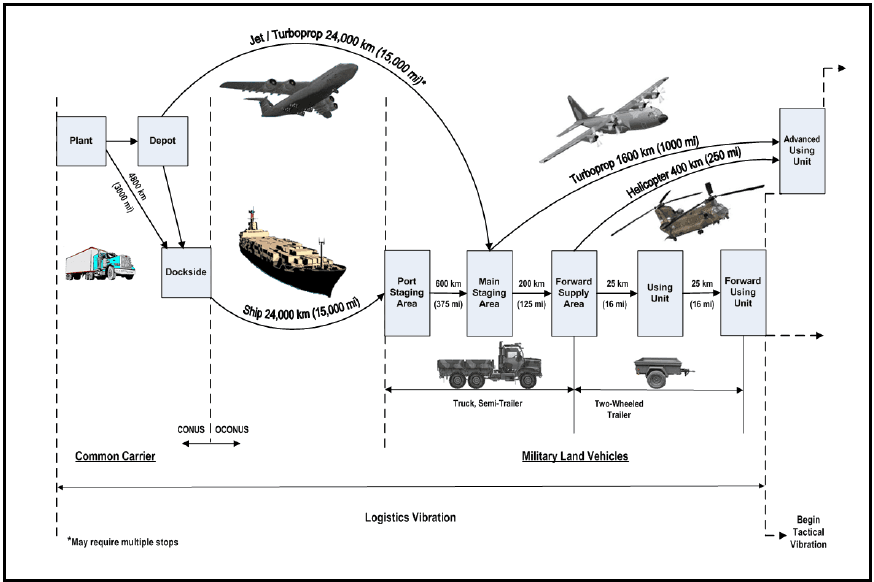
Figure description:
Typical Mission / Field Transportation Scenario
| Transport Segment | From | To | Distance (km) | Distance (mi) | Transport Mode |
|---|---|---|---|---|---|
| Common Carrier | Plant | Dockside | 4,800 | 3,000 | Truck / Semi-Trailer |
| Plant / Depot | Main Staging Area | 24,000 | 15,000* | Jet / Turboprop | |
| Dockside | Port Staging Area | 24,000 | 15,000 | Ship | |
| Military Land Vehicles | Port Staging Area | Main Staging Area | 600 | 375 | Truck, Semi-Trailer |
| Main Staging Area | Forward Supply Area | 200 | 125 | Truck, Semi-Trailer | |
| Forward Supply Area | Advanced Using Unit | 1,600 | 1,000 | Turboprop | |
| Forward Supply Area | Advanced Using Unit | 400 | 250 | Helicopter | |
| Forward Supply Area | Using Unit | 25 | 16 | Two-Wheeled Trailer | |
| Using Unit | Forward Using Unit | 25 | 16 | Two-Wheeled Trailer |
Key Details:
- Operational Boundary: Transition from CONUS to OCONUS occurs at the Dockside/Port Staging boundary.
- Logistics Scope: The diagram covers the "Logistics Vibration" phase, which transitions to "Tactical Vibration" after the Forward Using Unit.
- Note: Air transport of 24,000 km may require multiple stops.
Figure 514.8C-1. Typical mission / field transportation scenario.¹ 2
^1See paragraph 6.1, reference nm.
²In the event that tracked vehicles are identified in LCEP, they should be considered in the typical mission/field transportation scenario. See paragraph 6.1, reference d.
NOTE: This Figure represents only one mission in the life cycle of materiel. Determine the number of missions in the life cycle of the materiel from the LCEP. See Part One Paragraph 4.1.2c for Whole Life Assessment (WLA) and In Service Surveillance (ISS) considerations.
514.8-2 OPERATIONAL SERVICE
This paragraph applies to materiel installed in a vehicle, aircraft store, turbine engine, or carried by personnel. Such materiel may be permanently installed or removable.
514.8-2 SUPPLEMENTAL TESTS
2.1 Supplemental Considerations.
514.8-2 REQUIREMENTS
VSD requires a thorough knowledge of the dynamic environment in which the test hardware will be exposed when fielded. This knowledge must include characterization of the exposure levels and durations for all relevant conditions. Annex F, Appendix A presents guidelines and cautionary notes related to data acquisition.
Vibration of an item may be induced by transportation on a given platform, co-location near other vibrating equipment, self-induced, or a result of other sources. This annex is relevant as long as the expected exposure conditions and durations are understood, and the vibration levels can be measured and/or characterized.
To characterize the exposure levels, the test hardware and deployment vehicle (if applicable) are often instrumented at points of interest. The hardware is then exposed to the environments of concern and vibration data is acquired. In the event that the test items, prototypes, or carrier vehicles are not available, predictions of the vibration environment may be developed per simulation techniques provided the model fidelity is understood and has been properly verified and validated.
The duration of the vibration environments can be derived from the item’s Life Cycle Environment Profile (LCEP).
The life cycle will include many different types of induced mechanical environments which may occur while the materiel is being handled, transported, deployed and operated. Although all the induced mechanical environments are not critical in terms of generating potential damaging response amplitudes, they contribute in varying degrees to the materiel’s fatigue damage. All expected exposure conditions should be tabulated, along with corresponding durations, to form the items lifetime “scenario”. The scenario is a key parameter in the development of any vibration schedule. Methods for deriving an LCEP are discussed in Part 1 of this standard and in AECTP-100 (reference a). Methods for refining a scenario for VSD are presented in this annex.
514.8-2 VEHICLE PREPARATION FOR DATA ACQUISITION - CARGO
2.1 Specified Load: If the load and tie-down method are specified, no further instructions are necessary.
2.2 General Cargo Simulated Load: For general applications when loads and tie-down methods are not specified, choose typical cargo packages such as boxes, drums or cartons, designed to provide a simulated load that covers as much of the cargo bed as possible, consistent with the tie-down method. The cargo weight should be approximately 75 percent of the rated payload. This weight limitation is an arbitrary figure based on a study (reference j) in, which load weights were found to vary in the field enough to be unpredictable but tended toward full load. Another study revealed that the severity of the cargo bed vibration environment was minimal at full load and increased dramatically as the load decreased (reference k). The value of 75 percent of rated payload was chosen to provide a degree of conservatism. The analyst should consider the mission scenario carefully to establish the likelihood of lighter loads being carried. If unable to be reasonably sure that light loads will not be carried, some data capture should also be conducted using additional light load conditions and the VSD should utilize data from all load conditions considered.
Large rigid items such as steel plates, beams, concrete blocks, should not be used as simulated loads because their monolithic nature inhibits the flexibility of the cargo bed. In addition loose material such as sand or soil should not be placed directly on to the load bed as this will tend to dampen out any structural resonances present in the load floor.
2.3 Tie-down: The simulated load must be securely attached to the vehicle cargo bed using steel banding, web strapping, and/or dunnage. It must be secure enough to prevent movement between load and bed.
2.4 Accelerometers. Transducers must be mounted on the structural members of the cargo bed at locations that measure the input acceleration forces imparted to the load if an input control strategy is to be employed. If a response control strategy is planned then accelerometers should be mounted on structurally stiff locations at the base of the package or items being transported. The number of locations must be sufficient to describe the cargo bed environment. Care should be taken to avoid placing accelerometers in inappropriate places, i.e., the relatively thin steel plate that comprises most cargo bed surfaces.
514.8-2 STATISTICAL CONSIDERATIONS FOR DEVELOPING LIMITS ON AN ENSEMBLE OF DATA
This paragraph provides information relative to the statistical characterization of a set of data for the purpose of defining an upper limit of the data set related to statistical/probabilistic considerations. This section is based on the summary of work in reference g and is summarized in Method 516.8, Annex B.
Information in this paragraph is generally applicable to frequency domain estimates that are either predicted based on given information or time domain measurements processed in the frequency domain according to an appropriate technique i.e., for stationary random vibration, the processing would be an ASD; for a very short transient the processing could be a Shock Response Spectrum (SRS), an Energy Spectral Density (ESD), or a Fourier Spectrum (FS). Given estimates in the frequency domain, information in this Appendix will allow the establishment of upper limits of the data in a statistically correct way.
514.8-2 EXAMPLE APPLICATION OF FATIGUE DAMAGE SPECTRUM
Historically, four specific test courses at Aberdeen Test Center (ATC) have been used to generate data for vibration specifications for wheeled vehicles. It is improbable to relate the actual amount of each of these road surfaces to any real world scenario (e.g., determine how much Belgian Block a vehicle will encounter for a particular scenario), however it is possible to compute exposure times for operations at ATC and use this information to compute a fatigue damage spectrum by test course. Substantial precedence for using these course and speeds in full vehicle tests exists (first introduced as Large Assembly Transport Test of MIL-STD-810B, June 1967), so it is logical to use them as a basis for simulation. Each course has a measured length and is traversed at a nominal speed, leading to an exposure time. This information is presented in Table 514.8F-C.I.
| Test Course | |||
|---|---|---|---|
| Length, m (ft) | Nominal Speed, km/hr (mph) | Exposure Time, sec | |
| Belgian Block | 1200 (3940) | 32.2 (20) | 134 |
| Two-Inch Washboard | 250 (822) | 16.2 (10) | 56 |
| Radial Washboard | 74 (243) | 24.1 (15) | 11 |
| Three Inch Spaced Bump | 233 (764) | 32.2 (20) | 26 |
| Total | 1757 (5769) | 227 |
The exposure times can be used with equation C.1 and the appropriate test course ASDs to produce a fatigue damage spectrum for each test course. Using the same set of typical wheeled vehicle data as before, the fatigue spectra are shown in Figure 514.8F-C.1. For this example, was chosen to be 0.05 (5-percent critical damping) and the exponent was substituted for , and was assigned a value of 7.5 .
MIL-STD-810H METHOD 514.8, ANNEX F, APPENDIX C
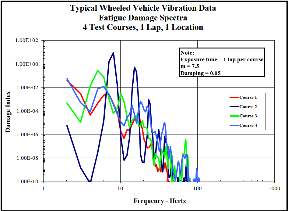
Figure description:
Typical Wheeled Vehicle Vibration Data 4 Test Courses, 1 Lap, 1 Location
Fatigue Damage Spectra
Legend
- Course 1 — color: red; symbol: Solid line
- Course 2 — color: dark blue; symbol: Solid line
- Course 3 — color: green; symbol: Solid line
- Course 4 — color: light blue; symbol: Solid line
Annotations
- Exposure time = 1 lap per course (text_label - position: x = 40, y = 1.00E+01)
- m = 7.5 (text_label - position: x = 40, y = 1.00E+00)
- Damping = 0.05 (text_label - position: x = 40, y = 1.00E-01)
| Frequency - Hertz | Course 1 | Course 2 | Course 3 | Course 4 |
|---|---|---|---|---|
| 2 | 5.00E-02 | 6.00E-06 | 5.00E-04 | 6.00E-02 |
| 3 | 5.00E-03 | 2.00E-08 | 1.00E-05 | 5.00E-04 |
| 4 | 4.00E-05 | 1.00E-10 | 2.00E-03 | 2.00E-04 |
| 5 | 5.00E-04 | 1.00E-08 | 3.00E-01 | 8.00E-03 |
| 6 | 1.00E-03 | 5.00E-06 | 1.00E-01 | 1.00E-02 |
| 7 | 2.00E-03 | 2.00E+00 | 2.00E-04 | 1.00E-02 |
| 8 | 3.00E-03 | 1.00E+01 | 6.00E-05 | 3.00E-03 |
| 9 | 1.00E-03 | 3.00E-01 | 1.00E-04 | 5.00E-04 |
| 10 | 1.00E-04 | 2.00E-04 | 3.00E-03 | 1.00E-05 |
| 15 | 2.00E-06 | 5.00E-01 | 1.00E-05 | 3.00E-04 |
| 20 | 2.00E-07 | 5.00E-09 | 1.00E-05 | 1.00E-04 |
| 25 | 1.00E-07 | 1.00E-03 | 3.00E-07 | 3.00E-04 |
| 30 | 1.00E-09 | 1.00E-06 | 2.00E-08 | 1.00E-07 |
| 40 | 1.00E-10 | 1.00E-08 | 1.00E-07 | 1.00E-05 |
| 50 | null | 1.00E-10 | 1.00E-09 | 5.00E-09 |
| 70 | null | 2.00E-09 | 4.00E-07 | 2.00E-08 |
| 100 | null | 1.00E-10 | 1.00E-10 | 1.00E-09 |
Notes: The chart uses logarithmic scales for both the X-axis (Frequency in Hertz and the Y-axis (Damage Index. The data values in the markdown table are estimates derived from the plot. Exposure time, m factor, and damping ratio are specified in a note within the chart area.))
Figure 514.8F-C.1. Fatigue damage spectra for specific test courses.
The cumulative fatigue damage spectrum (equation C.2) is shown by the lavender line in Figure 514.8F-C.2 and represents a fatigue damage index derived from a complete lap of the four specified test courses.
MIL-STD-810H METHOD 514.8, ANNEX F, APPENDIX C
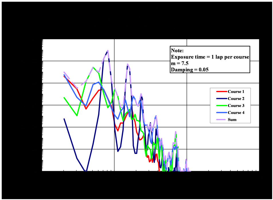
Figure description:
Typical Wheeled Vehicle Vibration Data 4 Test Courses, 1 Lap, 1 location
Fatigue Damage Spectra
Legend
- Course 1 — color: red; symbol: Solid line
- Course 2 — color: dark blue; symbol: Solid line
- Course 3 — color: bright green; symbol: Solid line
- Course 4 — color: light blue; symbol: Solid line
- Sum — color: light purple; symbol: Solid line
Annotations
- Note: Exposure time = 1 lap per course, m = 7.5, Damping = 0.05 (text_label - position: top right)
| Frequency (Hertz) | Course 1 | Course 2 | Course 3 | Course 4 | Sum |
|---|---|---|---|---|---|
| 2 | 5.00E-02 | 6.00E-06 | 5.00E-04 | 5.00E-02 | 1.00E-01 |
| 3 | 1.00E-02 | 2.00E-09 | 1.00E-05 | 5.00E-03 | 1.50E-02 |
| 4 | 5.00E-05 | 1.00E-10 | 2.00E-02 | 1.00E-04 | 2.00E-02 |
| 5 | 1.00E-03 | 3.00E-08 | 2.00E-01 | 8.00E-03 | 2.10E-01 |
| 6 | 2.00E-03 | 1.00E-06 | 8.00E-02 | 1.20E-02 | 9.50E-02 |
| 7 | 3.00E-03 | 1.00E-01 | 1.00E-04 | 5.00E-03 | 1.10E-01 |
| 8 | 1.00E-03 | 8.00E+00 | 5.00E-04 | 2.00E-03 | 8.00E+00 |
| 9 | 5.00E-04 | 1.00E+00 | 1.00E-04 | 5.00E-04 | 1.00E+00 |
| 10 | 1.00E-05 | 1.00E-04 | 2.00E-03 | 1.00E-04 | 2.20E-03 |
| 12 | 1.00E-05 | 2.00E-03 | 5.00E-04 | 2.00E-04 | 2.70E-03 |
| 15 | 5.00E-05 | 1.00E+00 | 1.00E-04 | 3.00E-04 | 1.00E+00 |
| 20 | 1.00E-05 | 1.00E-05 | 1.00E-05 | 6.00E-04 | 6.30E-04 |
| 25 | 2.00E-07 | 5.00E-04 | 2.00E-06 | 2.00E-04 | 7.00E-04 |
| 30 | 1.00E-08 | 2.00E-06 | 1.00E-07 | 2.00E-06 | 4.10E-06 |
| 40 | 1.00E-09 | 1.00E-05 | 1.00E-07 | 1.00E-05 | 2.00E-05 |
| 50 | 1.00E-10 | 2.00E-09 | 5.00E-10 | 2.00E-09 | 5.00E-09 |
| 60 | 1.00E-10 | 1.00E-09 | 1.00E-09 | 2.50E-08 | 2.70E-08 |
| 70 | 1.00E-10 | 4.00E-07 | 3.00E-07 | 1.50E-08 | 7.20E-07 |
| 80 | 1.00E-10 | 1.00E-10 | 1.00E-10 | 1.00E-10 | 1.00E-10 |
| 100 | 1.00E-10 | 1.00E-10 | 1.00E-10 | 1.00E-10 | 1.00E-10 |
Notes: The data represents a Fatigue Damage Spectra (FDS for four test courses. Both axes are on a logarithmic scale. The Y-axis represents Damage index and the X-axis represents Frequency in Hertz.)
Figure 514.8F-C.2. Cumulative fatigue damage spectrum (lavender line).
The same process was performed for 2 measurement locations independently using cumulative data for 3 laps. The cumulative spectra for each location were then averaged and enveloped for comparison and are shown in Figure 514.8F-C.3.
MIL-STD-810H METHOD 514.8, ANNEX F, APPENDIX C
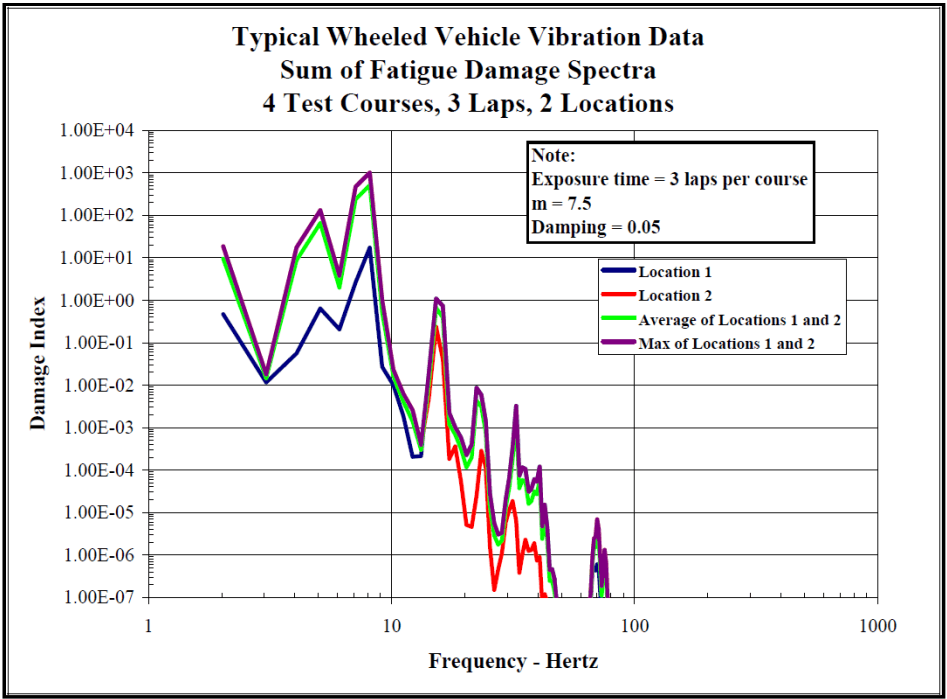
Figure description:
Typical Wheeled Vehicle Vibration Data Sum of Fatigue Damage Spectra 4 Test Courses, 3 Laps, 2 Locations
Sum of Fatigue Damage Spectra
Legend
- Location 1 — color: dark blue; symbol: solid line
- Location 2 — color: red; symbol: solid line
- Average of Locations 1 and 2 — color: light green; symbol: solid line
- Max of Locations 1 and 2 — color: purple; symbol: solid line
Annotations
- Note: Exposure time = 3 laps per course m = 7.5 Damping = 0.05 (text_label - position: top right of plot area
| Frequency - Hertz | Location 1 | Location 2 | Average of Locations 1 and 2 | Max of Locations 1 and 2 |
|---|---|---|---|---|
| 2.0 | 4.70E-01 | 1.80E+01 | 9.24E+00 | 1.80E+01 |
| 3.0 | 1.10E-02 | 1.50E-02 | 1.30E-02 | 1.50E-02 |
| 4.0 | 5.50E-02 | 1.60E+01 | 8.03E+00 | 1.60E+01 |
| 5.0 | 6.50E-01 | 1.40E+02 | 7.03E+01 | 1.40E+02 |
| 6.0 | 2.00E-01 | 3.50E+00 | 1.85E+00 | 3.50E+00 |
| 8.0 | 1.80E+01 | 9.50E+02 | 4.84E+02 | 9.50E+02 |
| 10.0 | 2.50E-02 | 5.50E-02 | 4.00E-02 | 5.50E-02 |
| 12.0 | 2.10E-04 | 8.00E-04 | 5.05E-04 | 8.00E-04 |
| 14.0 | 5.00E-01 | 1.20E-01 | 3.10E-01 | 5.00E-01 |
| 15.0 | 1.10E+00 | 2.50E-01 | 6.75E-01 | 1.10E+00 |
| 17.0 | 1.00E-03 | 1.50E-04 | 5.75E-04 | 1.00E-03 |
| 20.0 | 2.00E-04 | 5.00E-06 | 1.03E-04 | 2.00E-04 |
| 23.0 | 9.00E-03 | 3.00E-04 | 4.65E-03 | 9.00E-03 |
| 27.0 | 1.00E-06 | 1.40E-07 | 5.70E-07 | 1.00E-06 |
| 30.0 | 2.00E-05 | 1.50E-06 | 1.08E-05 | 2.00E-05 |
| 33.0 | 3.30E-03 | 2.00E-05 | 1.66E-03 | 3.30E-03 |
| 37.0 | 1.00E-04 | 1.50E-06 | 5.08E-05 | 1.00E-04 |
| 40.0 | 1.20E-04 | 2.10E-06 | 6.11E-05 | 1.20E-04 |
| 45.0 | 5.00E-07 | null | 2.50E-07 | 5.00E-07 |
| 75.0 | 7.00E-06 | 2.00E-07 | 3.60E-06 | 7.00E-06 |
| 85.0 | 1.00E-07 | null | null | 1.00E-07 |
Notes: The Y-axis (Damage Index and X-axis (Frequency - Hertz are both on logarithmic scales. Data points were estimated based on the log-log grid provided.))
Figure 514.8F-C.3. Cumulative fatigue spectra from locations 1 and 2.
If an overall exposure time is selected, equation C.1 can be reworked to provide an ASD level based on the fatigue spectrum computed from Equation C.2.
C.3
| where: | |
|---|---|
| DP(fn) = | Cumulative damage index as a function of system natural frequency |
| fn = | System natural frequency (variable), Hz |
| T = | Total exposure time in environment, seconds |
| G(fn) = | Equivalent ASD for a given DP(fn), T, g2/Hz |
| ζ = | Damping ratio of system at dominant natural frequency expressed as a decimal |
| b = | Fatigue curve slope value when computed as a linear fit in log-log domain. |
MIL-STD-810H METHOD 514.8, ANNEX F, APPENDIX C
Using an exposure time equal to 3 times the total value listed in Table 514.8F-C.I (to account for 3 laps) and the fatigue damage spectra (average and max) shown in Figure 514.8F-C.3, an equivalent representative ASD was calculated from equation C.3. The spectra derived from the average and maximum fatigue damage spectra are shown in Figure 514.8F-C.4. For this data set, the fatigue damage spectra for locations 1 and 2 were nearly the same producing an average spectrum that is about the same as the enveloped spectrum. The enveloped or maximum spectrum is compared to the resultant spectrum computed from the statistical process and from a spectrum derived from the envelope of all original spectra and is shown in Figure 514.8F-C.5.
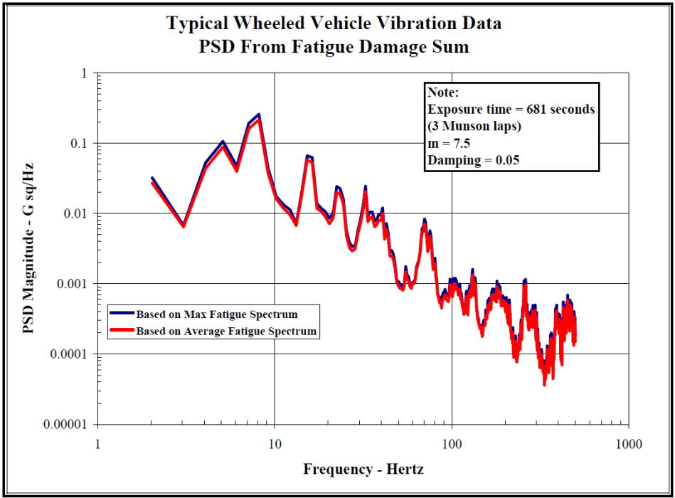
Figure description:
Typical Wheeled Vehicle Vibration Data PSD From Fatigue Damage Sum
PSD From Fatigue Damage Sum
Legend
- Based on Max Fatigue Spectrum — color: blue; symbol: Solid line
- Based on Average Fatigue Spectrum — color: red; symbol: Solid line
Annotations
- Note: Exposure time = 681 seconds (3 Munson laps m = 7.5 Damping = 0.05 (text_label - position: top right of graph area))
| Frequency - Hertz | Based on Max Fatigue Spectrum (G sq/Hz) | Based on Average Fatigue Spectrum (G sq/Hz) |
|---|---|---|
| 2.0 | 0.033 | 0.027 |
| 3.0 | 0.007 | 0.0065 |
| 4.0 | 0.054 | 0.048 |
| 5.0 | 0.107 | 0.092 |
| 6.0 | 0.046 | 0.039 |
| 7.1 | 0.198 | 0.176 |
| 8.0 | 0.264 | 0.233 |
| 9.5 | 0.036 | 0.028 |
| 10.3 | 0.017 | 0.015 |
| 13.5 | 0.009 | 0.0068 |
| 15.3 | 0.068 | 0.061 |
| 17.5 | 0.013 | 0.011 |
| 20.3 | 0.0089 | 0.0074 |
| 23.0 | 0.024 | 0.021 |
| 27.5 | 0.0035 | 0.0031 |
| 35.0 | 0.025 | 0.022 |
| 40.5 | 0.0071 | 0.0063 |
| 50.5 | 0.012 | 0.0094 |
| 62.0 | 0.0011 | 0.00086 |
| 71.0 | 0.0083 | 0.0071 |
| 95.0 | 0.0011 | 0.00092 |
| 104.0 | 0.0012 | 0.0011 |
| 130.0 | 0.0016 | 0.0013 |
| 160.0 | 0.00042 | 0.00033 |
| 185.0 | 0.0010 | 0.00085 |
| 235.0 | 0.00018 | 0.00014 |
| 265.0 | 0.0011 | 0.00095 |
| 320.0 | 0.000078 | 0.000057 |
| 420.0 | 0.00068 | 0.00052 |
| 500.0 | 0.00042 | 0.00031 |
Notes: The chart uses a logarithmic scale for both axes. Frequency ranges from 1 to 1000 Hertz, and PSD Magnitude ranges from 0.00001 to 1 G sq/Hz.
Figure 514.8F-C.4. Combined vibration power spectra developed from average and maximum fatigue damage Spectra.
MIL-STD-810H METHOD 514.8, ANNEX F, APPENDIX C
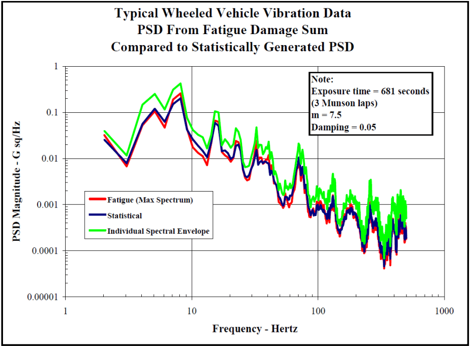
Figure description:
Typical Wheeled Vehicle Vibration Data PSD From Fatigue Damage Sum Compared to Statistically Generated PSD
Legend
- Fatigue (Max Spectrum — color: red; symbol: Solid line
- Statistical — color: dark blue; symbol: Solid line
- Individual Spectral Envelope — color: green; symbol: Solid line
Annotations
- Note: Exposure time = 681 seconds (3 Munson laps, m = 7.5, Damping = 0.05 (text_label - position: top right))
| Frequency - Hertz | Fatigue (Max Spectrum - PSD Magnitude (G sq/Hz)) | Statistical - PSD Magnitude (G sq/Hz) | Individual Spectral Envelope - PSD Magnitude (G sq/Hz) |
|---|---|---|---|
| 2.0 | 0.03 | 0.025 | 0.04 |
| 3.0 | 0.007 | 0.008 | 0.012 |
| 4.0 | 0.05 | 0.045 | 0.14 |
| 5.0 | 0.11 | 0.11 | 0.25 |
| 6.5 | 0.05 | 0.06 | 0.11 |
| 7.5 | 0.15 | 0.13 | 0.3 |
| 8.5 | 0.26 | 0.21 | 0.42 |
| 10.0 | 0.017 | 0.025 | 0.043 |
| 15.0 | 0.07 | 0.065 | 0.105 |
| 18.0 | 0.013 | 0.015 | 0.026 |
| 23.0 | 0.025 | 0.02 | 0.047 |
| 30.0 | 0.0035 | 0.004 | 0.006 |
| 37.0 | 0.02 | 0.009 | 0.048 |
| 55.0 | 0.001 | 0.0009 | 0.002 |
| 70.0 | 0.007 | 0.006 | 0.021 |
| 100.0 | 0.0006 | 0.0007 | 0.0023 |
| 135.0 | 0.001 | 0.001 | 0.0048 |
| 170.0 | 0.00025 | 0.0003 | 0.0012 |
| 210.0 | 0.0008 | 0.0006 | 0.0018 |
| 250.0 | 0.0001 | 0.00015 | 0.00035 |
| 290.0 | 0.0003 | 0.0002 | 0.0035 |
| 350.0 | 0.00004 | 0.00006 | 0.00012 |
| 420.0 | 0.0003 | 0.00025 | 0.0015 |
| 500.0 | 0.0002 | 0.00015 | 0.0008 |
Notes: The chart is a log-log plot representing PSD Magnitude vs. Frequency for wheeled vehicle vibration data.
Figure 514.8F-C.5. Comparison of combined vibration power spectrum developed from the fatigue damage
spectrum, from the statistical process and from an envelope process.
The three processes (fatigue spectrum, statistical and envelope) produce specifications that are roughly the same shape. The specification derived from the fatigue damage spectrum technique has lower levels than those produced by the envelope process and nearly the same (but generally lower) levels than those produced by the technique developed in Appendix B. The statistical technique contains an implied assumption that each environment has the same exposure time and weights the spectral values toward the most severe spectrum due to the inclusion of spectral variance (the addition of a standard deviation) in the process. Therefore, it is likely that the statistical process will produce higher levels than the fatigue damage process unless the most severe spectra also have the longest exposure times.
The process was repeated for an exponent value of m = 5 as a comparison. A comparison of the fatigue damage spectra (maximum) for the two exponents is shown in Figure 514.8F-C.6, and a comparison of the vibration power spectra developed from each exponent is presented in Figure 514.8F-C.7.
MIL-STD-810H METHOD 514.8, ANNEX F, APPENDIX C
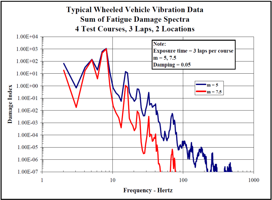
Figure description:
Typical Wheeled Vehicle Vibration Data Sum of Fatigue Damage Spectra, 4 Test Courses, 3 Laps, 2 Locations
Sum of Fatigue Damage Spectra
Legend
- m = 5 — color: blue; symbol: Solid line
- m = 7.5 — color: red; symbol: Solid line
Annotations
- Note: Exposure time = 3 laps per course, m = 5, 7.5, Damping = 0.05 (text_label - position: top right of plot area)
| Frequency - Hertz | m = 5 | m = 7.5 |
|---|---|---|
| 2.0 | 6.50E+01 | 1.80E+01 |
| 3.0 | 7.00E-01 | 1.80E-02 |
| 5.0 | 1.40E+02 | 1.10E+02 |
| 6.5 | 2.00E+01 | 4.00E+00 |
| 8.0 | 1.00E+03 | 1.10E+03 |
| 10.0 | 5.00E-01 | 2.00E-02 |
| 13.0 | 6.00E-02 | 4.00E-04 |
| 15.0 | 1.50E+01 | 1.10E+00 |
| 20.0 | 6.00E-02 | 2.20E-04 |
| 25.0 | 6.00E-01 | 1.00E-02 |
| 35.0 | 3.00E-01 | 3.50E-03 |
| 40.0 | 2.50E-02 | 3.50E-05 |
| 45.0 | 3.50E-02 | 1.20E-04 |
| 55.0 | 4.00E-05 | null |
| 70.0 | 5.00E-03 | 7.00E-06 |
| 80.0 | 1.50E-03 | 1.00E-06 |
| 100.0 | 3.00E-05 | null |
| 130.0 | 3.00E-05 | null |
| 145.0 | 5.00E-06 | null |
| 180.0 | 1.00E-05 | null |
| 250.0 | 3.50E-06 | null |
| 300.0 | 4.00E-07 | null |
| 400.0 | 2.50E-07 | null |
| 480.0 | 6.00E-07 | null |
Notes: The x-axis (Frequency in Hertz and y-axis (Damage Index both use logarithmic scales. Data points represent the sum of fatigue damage spectra for 4 test courses, 3 laps, and 2 locations.))
Figure 514.8F-C.6. Fatigue damage spectra for two exponents.
MIL-STD-810H METHOD 514.8, ANNEX F, APPENDIX C
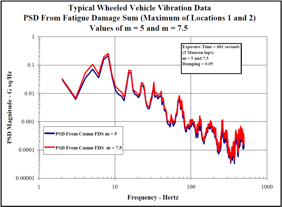
Figure description:
Typical Wheeled Vehicle Vibration Data", "subtitle": "PSD From Fatigue Damage Sum (Maximum of Locations 1 and 2\nValues of m = 5 and m = 7.5", "additional_notes": "The axes are on a logarithmic scale. Data values are estimated from the graph grid lines and represent key peaks and troughs to capture the profile of the fatigue damage sum spectrum. Red (m=7.5 shows higher sensitivity to peak values compared to blue (m=5.
PSD From Fatigue Damage Sum (Maximum of Locations 1 and 2
Legend
- PSD From Cumm FDS m = 5 — color: blue; symbol: Solid line
- PSD From Cumm FDS m = 7.5 — color: red; symbol: Solid line
Annotations
- Exposure Time = 681 seconds, (3 Munson laps, m = 5 and 7.5, Damping = 0.05 (text_label - position: top right box))
| Frequency - Hertz | PSD From Cumm FDS m = 5 | PSD From Cumm FDS m = 7.5 |
|---|---|---|
| 2.0 | 0.030 | 0.033 |
| 3.1 | 0.006 | 0.007 |
| 4.8 | 0.070 | 0.100 |
| 7.8 | 0.200 | 0.250 |
| 10.0 | 0.013 | 0.018 |
| 12.0 | 0.005 | 0.007 |
| 15.0 | 0.055 | 0.065 |
| 19.0 | 0.007 | 0.010 |
| 22.0 | 0.019 | 0.024 |
| 28.0 | 0.003 | 0.004 |
| 30.0 | 0.008 | 0.024 |
| 40.0 | 0.008 | 0.012 |
| 50.0 | 0.0008 | 0.0012 |
| 60.0 | 0.0008 | 0.0015 |
| 70.0 | 0.0055 | 0.0080 |
| 100.0 | 0.0005 | 0.0008 |
| 150.0 | 0.0008 | 0.0015 |
| 180.0 | 0.0006 | 0.0010 |
| 250.0 | 0.0007 | 0.0011 |
| 300.0 | 0.0002 | 0.0004 |
| 400.0 | 0.0002 | 0.0005 |
| 500.0 | 0.00015 | 0.0003 |
Figure 514.8F-C.7. Comparison of combined vibration power spectra developed from two exponents.
For this set of measured environments (acceleration spectra) and associated exposure times, the final combined spectrum is somewhat independent of the value of the exponent chosen. Forty percent of the spectral amplitudes for the two exponents were within 1 dB (based on m=7.5 as the reference), 80 percent were within 2 dB and all were within 2.4 dB.
Documentation of the spectral combination process, including assumptions (e.g., value of b), is essential. The final combined spectrum should be compared to the original input spectra to ensure that the resultant spectrum is a reasonable representation of the measured environment.
- FDS APPROACH TO DEVELOPMENT OF A LVTS.
In summarizing the example provided in the previous section, a single ASD was computed, representative of the ensemble of data acquired from making three passes over four specific road courses. The ASD derived from the inverse of the cumulative FDS is compared to the envelope of the data ensemble as shown in Figure 514.8F-C.5. From Figure 514.8F-C.7 it is clear that the spectral shapes and amplitudes are very similar for the ASD’s derived in the examples in previous section for both selections of m (m=5 and m=7.5). From Figure 514.8F-C.5 it is also clear that the ASD computed from the inverse cumulative FDS falls significantly below the envelope of the data ensemble. Employing equation 9.5, one could easily compress the test time by increasing the magnitude of the ASD. This can be accomplished by changing the T parameter of equation C.3. As in Annex F, paragraph 9, one should always use caution in employing time compression techniques. When dealing with data of a similar spectral characteristic, a conservative approach would be to limit the final compressed spectral shape to the spectral shape of the envelope of the original data ensemble. Reviewing the spectral shapes of the ASD’s computed from the inverse cumulative FDS and the envelope of the original data ensemble, it is clear that the ratio between the two curves is not the same at each spectral line. Therefore, one will need to set some criteria, which is often test specific, for addressing the amount of
MIL-STD-810H METHOD 514.8, ANNEX F, APPENDIX C
time compression employed. In the example discussed in this Appendix, the average ratio between 2 and 100 Hz was set at the compression ratio. This spectral band was considered to be of primary importance for this example since the data set was from a wheeled vehicle and the spectrum is dominated by energy below 100 Hz. Figure 514.8F-C.8 illustrates the effect of time compression based on the ratio described above. Using the time compressed spectral shape, the test time reduces from 681 seconds (the actual time spent on the courses) to either 72 seconds (when ) or 54 seconds (when ). As a final step, the analyst will usually reduce the number of breakpoints (smooth the spectral shape) while maintaining the overall G-rms level.
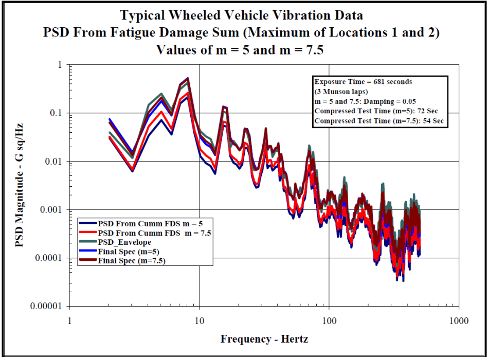
Figure description:
Typical Wheeled Vehicle Vibration Data Values of m = 5 and m = 7.5
PSD From Fatigue Damage Sum (Maximum of Locations 1 and 2
Legend
- PSD From Cumm FDS m = 5 — color: dark blue; symbol: solid line
- PSD From Cumm FDS m = 7.5 — color: red; symbol: solid line
- PSD_Envelope — color: teal; symbol: solid line
- Final Spec (m=5 — color: blue; symbol: solid line
- Final Spec (m=7.5 — color: dark red; symbol: solid line
Annotations
- Exposure Time = 681 seconds (3 Munson laps (text_label - position: top right box))
- m = 5 and 7.5; Damping = 0.05 (text_label - position: top right box)
- Compressed Test Time (m=5: 72 Sec (text_label - position: top right box))
- Compressed Test Time (m=7.5: 54 Sec (text_label - position: top right box))
| Frequency - Hertz | PSD From Cumm FDS m = 5 | PSD From Cumm FDS m = 7.5 | PSD_Envelope | Final Spec (m=5) | Final Spec (m=7.5) |
|---|---|---|---|---|---|
| 2.0 | 0.035 | 0.04 | 0.04 | 0.075 | 0.065 |
| 3.0 | 0.006 | 0.008 | 0.012 | 0.015 | 0.012 |
| 5.0 | 0.04 | 0.07 | 0.15 | 0.1 | 0.08 |
| 7.0 | 0.07 | 0.1 | 0.25 | 0.2 | 0.15 |
| 8.0 | 0.08 | 0.2 | 0.5 | 0.25 | 0.4 |
| 10.0 | 0.012 | 0.018 | 0.045 | 0.035 | 0.03 |
| 13.0 | 0.005 | 0.008 | 0.025 | 0.02 | 0.015 |
| 15.0 | 0.06 | 0.1 | 0.14 | 0.12 | 0.11 |
| 18.0 | 0.01 | 0.015 | 0.025 | 0.02 | 0.018 |
| 23.0 | 0.025 | 0.035 | 0.05 | 0.045 | 0.04 |
| 30.0 | 0.003 | 0.004 | 0.008 | 0.006 | 0.005 |
| 32.0 | 0.015 | 0.02 | 0.05 | 0.04 | 0.035 |
| 40.0 | 0.007 | 0.01 | 0.025 | 0.018 | 0.015 |
| 50.0 | 0.0008 | 0.0012 | 0.0035 | 0.0025 | 0.002 |
| 60.0 | 0.0007 | 0.001 | 0.003 | 0.002 | 0.0015 |
| 70.0 | 0.005 | 0.008 | 0.02 | 0.015 | 0.012 |
| 80.0 | 0.0006 | 0.0009 | 0.002 | 0.0015 | 0.0012 |
| 100.0 | 0.0004 | 0.0006 | 0.0025 | 0.002 | 0.0015 |
| 130.0 | 0.001 | 0.0015 | 0.005 | 0.0035 | 0.0025 |
| 200.0 | 0.0001 | 0.0002 | 0.002 | 0.0015 | 0.001 |
| 250.0 | 0.0005 | 0.0008 | 0.0035 | 0.0025 | 0.002 |
| 300.0 | 0.00004 | 0.00006 | 0.0015 | 0.001 | 0.0008 |
| 400.0 | 0.00006 | 0.0001 | 0.0018 | 0.0012 | 0.001 |
| 500.0 | 0.00015 | 0.00025 | 0.002 | 0.0015 | 0.0012 |
Notes: The y-axis is in a logarithmic scale for Power Spectral Density (G sq/Hz, and the x-axis is in a logarithmic scale for Frequency (Hz. Values in the table are approximate based on the plot.))
Figure 514.8F-C.8. Time compression of ASD's computed from the inverse cumulative fatigue damage spectrum.
This example is relatively simple; however, the techniques could easily be expanded to address more complex ensembles of data to include spectra with either narrowband or tonal components.
MIL-STD-810H METHOD 514.8, ANNEX F, APPENDIX D
Vibration Specification Development Procedure
514.8-2 BROADBAND PROFILE DEVELOPMENT
514.8-2 SINUSOIDAL EXCITATION
Given a sinusoidal excitation with the form:
The relative response displacement z(t) of a linear system with one degree of freedom is expressed:
-x(t) z(t) =
«³ {{² - ()]* + *()} ως 2)
For given values for f and fo, z(t) is a maximum when x(t) = x(m):
-x(m) MRS = wz(t) =
+452
The MRS is the curve representing the variations of ω 0 z 2 m versus f0, for given value of ξ. The positive and negative spectra are symmetric. The positive spectrum goes through a maximum when the denominator goes through a minimum, i.e.:
Xm MRS = 23√1-32
As an initial approximation, it can be considered that:
MRS = Qxm
Example: MRS for a fixed sine excitation at 500 Hz with Q=5 (Figure 514.8F-E.1).
MIL-STD-810H METHOD 514.8, ANNEX F, APPENDIX E
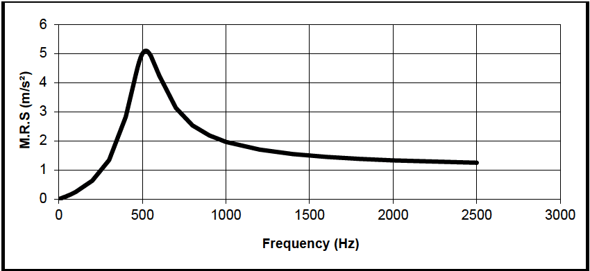
Figure description:
M.R.S vs Frequency
| Frequency (Hz) | M.R.S (m/s²) |
|---|---|
| 0 | 0.0 |
| 100 | 0.3 |
| 200 | 0.6 |
| 300 | 1.3 |
| 400 | 2.8 |
| 500 | 4.8 |
| 520 | 5.1 |
| 600 | 3.8 |
| 700 | 3.1 |
| 800 | 2.5 |
| 1000 | 2.0 |
| 1500 | 1.5 |
| 2000 | 1.35 |
| 2500 | 1.25 |
Notes: The data series represents a single response curve showing a peak M.R.S value of approximately 5.1 m/s² at a frequency of about 520 Hz. The chart features gridlines every 500 Hz on the x-axis and every 1 m/s² on the y-axis.
Figure 514.8F-E.1. MRS for a fixed sine excitation at 500 Hz with Q=5.
2.1 Selecting this Method
Essentially all materiel will experience vibration, whether during manufacture, transportation, maintenance, or operational use. The procedures of this Method address most of the life cycle situations during which vibration is likely to be experienced. Select the procedure or procedures most appropriate for the materiel to be tested and the environment to be simulated. See Table 514.8-I for a general listing of vibration exposures and test procedures as related to environmental life cycle elements. See Annexes B-F for guidance on determining vibration levels and durations.
- a. Fidelity of the laboratory test environment. As noted in Part I (Paragraph 1.3), laboratory test methods are limited in their abilities to simulate synergistic or antagonistic stress combinations, dynamic (time
MIL-STD-810H
METHOD 514.8
sequence) stress applications, aging, and other potentially significant stress combinations present in natural field/fleet service environments. Use caution when defining and extrapolating analyses, test criteria, and results. An assessment of the test article vulnerabilities should be used to determine the environmental variables that are essential to the laboratory test and potential for increased margin to compensate for deficiencies in the test environment. Reduction in test environment fidelity may lead to an increased risk to material life and function in the fielded environment.
- b. Conservatism with measured data. The guidance in this document encourages the use of materiel-specific measured data as the basis for vibration criteria. Due to limitations in numbers of transducers, accessibility of measurement points, linearity of data at extreme conditions, and other causes, measurements do not include all extreme conditions. Further, there are test limitations such as single axis versus multi-axis, and practical fixtures versus platform support. Apply margin to measured data in deriving test criteria to account for these variables. When sufficient measured data are available, use statistical methods as shown in Annex F.
- c. Conservatism with default or enveloped data. Annexes B - E of this Method provide information that can be used to generate default criteria for those cases where measured data are unavailable. These data are based on envelopes of wide ranges of cases and are conservative for any one case. Additional margin is not recommended. Use caution when conducting vibration test with default or enveloped vibration data if non-linear behavior is expected or observed at full test level. If non-linear behavior is a concern, a ramp up step should be added to the test schedule. The vibration amplitude of this additional ramp up step shall have an exaggeration factor of unity. This unity ramp up step duration should be at least 10 minutes. The data measured during full test level and the unity ramp up step can be used to evaluate the linearity of the materiel during accelerated test. If materiel is determined to behave non-linearly using the above technique, the organization responsible for the materiel under test shall be notified. Test options should be explored and a proposed path forward should be identified. The test options and proposed path forward should be sent to the appropriate test authority for concurrence prior to proceeding.
NOTE: The materiel's anticipated Life Cycle Environmental Profile (LCEP) may reveal other vibration scenarios that are not specifically addressed in the procedures. Tailor the procedures as necessary to capture the LCEP variations, but do not reduce the basic test requirements reflected in the below procedures without proper justification. (See paragraph 2.3 below.)
514.8-2.1 Vibration Test Types
The following presents discussions of general types of vibration tests. Other test types, definitions, and names will be found in practice. All of these test types may not be applied to a given materiel item. A typical materiel development might include development testing and durability testing, while another might include qualification and reliability testing. Environmental worthiness testing is included when needed. Environmental Stress Screening (ESS) is a part of most current DOD acquisitions. All of the tests, including ESS, consume vibratory fatigue life. In many cases, a qualification test, a durability test, or a reliability test consumes so much of the fatigue life of the test article that it is not suitable for field deployment. However, there are instances in which the same tests are conducted to only a portion of the fatigue life in the conduct of a system level version of an ESS test. Similarly, development tests and worthiness tests may or may not consume a complete life depending on the specific test goals. It is important to ensure ESS consumes only an appropriate, hopefully negligible, portion of total life, and that this portion is accounted for in the total life cycle of vibration exposures. In all cases, it is vital to tailor test methodology and requirements to achieve the desired results.
514.8-2.1 Category 1 - Manufacturing/Maintenance Processes
All materiel will experience some vibration during manufacture and maintenance. When different serial number items (lots) experience significant differences in vibration exposure during manufacture, select vibration test specimens, exposure levels, and exposure durations from those lots that experience the maximum vibration exposure. For maintenance, evaluate this environment and, when significant, include it in design and test exposures, along with the exposure levels and durations.
514.8-2.1 Category 4 - Truck/Trailer - Secured Cargo
These transportation environments are characterized by broadband vibration resulting from the interaction of vehicle suspension and structures with road and surface discontinuities. Representative conditions experienced on moving materiel from point of manufacture to end-use are depicted in Part One, Figure 1-4a. This environment may be divided into two phases, truck transportation over US highways, and mission/field transportation. Mission/field transportation is further broken down into two-wheeled trailer and wheeled vehicles categories.
2.1.1 Truck transportation over US highways. This involves movement from the manufacturer's plant to any continental United States storage or user installation. (Data are available for US roads, but not for roads in other countries.) This movement is usually accomplished by large truck and/or tractor-trailer combination. Mileage for this transportation generally ranges from 3200 to 6400 kilometers (2000 to 4000 miles) over improved or paved highways.
514.8-2.1 Category 12 - Fixed wing aircraft - jet aircraft
The vibration environment for materiel installed in jet aircraft (except engine-mounted (see paragraph 2.11 of this Annex)), and gunfire-induced, (see Method 519.8) stems from four principal mechanisms. These are (1) engine noise impinging on aircraft structures; (2) turbulent aerodynamic flow over external aircraft structures, (3) turbulent aerodynamic flow and acoustic resonance phenomena within cavities open to the external airflow, particularly open weapon bays, and (4) airframe structural motions due to maneuvers, aerodynamic buffet, landing, taxi, etc. Vibration can also be produced by installed materiel items. These vibrations are generally important only locally at or near the source and may not be significant even in that local area.
- a. Airframe structural response. Airframe structural motions are the responses of flexible airframe structures to transient events. Examples of such events are landing impact, arrested landings, catapult, rebound of wings and pylons when heavy stores are ejected, and separated flow or shed vortex excitation of flight surfaces during maneuvers. Catapult take-off and arrested landing also result in structural motions. These are included in Method 516.8 as transient vibrations. Airframe structural motions are most important for the outer regions of flexible structures (i.e., outer 1/2 of wings, empennage, pylons, etc.). These vibrations are characteristic of the particular airframe involved and must be evaluated through measured data. In other areas of the airframe (fuselage, inboard wing, etc.) these vibrations are relatively mild and are generally covered by the fallback criteria described below or by minimum integrity criteria (Annex E, paragraph 2.1).
- b. Jet noise and aerodynamically induced vibration. Jet noise induced vibration is usually dominant in vehicles that operate at lower dynamic pressures, i.e., limited to subsonic speeds at lower altitudes and transonic speeds at high altitudes (paragraph 6.1, reference i). Aerodynamically induced vibration usually predominates in vehicles that operate at transonic speeds at lower altitudes, or supersonic speeds at any altitude (paragraph 6.1, references j and k).
- c. Cavity noise induced vibration. Where there are openings in the aircraft skin with airflow across the
opening, the corresponding cavity within the aircraft is subject to very high levels of aerodynamic and acoustic fluctuating pressures. This is because of general flow disruption and, more importantly, to a phenomenon known as cavity resonance. The fluctuating pressures can be crudely predicted analytically (see paragraph 6.1, references l and m) and somewhat more accurately measured in wind tunnel measurements. Flight test measurement is the only accurate method available to determine these pressures. Further, given the pressures, it is very difficult to predict the resulting vibration and no simple method is available. This vibration should be measured. These vibrations are likely to be important in the local areas surrounding small cavities such as flare launchers, cooling air exhaust openings, etc. With large cavities (particularly weapons bays), the resulting vibration is likely to be a major element of the overall aircraft environment. Method 515.8 contains an acoustic test simulating this environment. That procedure may be used for materiel located inside the cavity, but it is not suitable for simulating the vibration environments for areas near the cavity. Where cavities remain open continuously, the vibration is continuous. When doors or covers open, there will be a transient vibration. While the doors remain open, there is a steady state vibration, followed by another transient vibration as the doors close. When doors open and close quickly, the entire event can sometimes be characterized as a single transient vibration.
- d. Materiel induced vibration. In addition, installed materiel can produce significant vibration. Any materiel that involves mechanical motion may produce vibration. This is particularly true of those that have rotating elements such as motors, pumps, and gearboxes. The vibration output of installed materiel varies widely and is highly dependent on the mounting as well as the characteristics of the materiel. There is no basis for predicting local environments due to materiel. Materiel items must be evaluated individually. General aircraft environments as discussed above can generally be expected to cover the contribution of installed materiel.
- e. Exposure levels. Vibration criteria in the form of qualification test levels (see Annex A, paragraph 2.1.2) have been established for most airplanes developed for the military. Obtain these criteria through the program office responsible for the particular aircraft. This is the recommended basis for developing exposure levels. In cases where satisfactory criteria are not available, measured data may be available through the aircraft program office. Otherwise, measurements of actual vibrations are recommended.
- (1) As a last resort, the guidance of Figure 514.8D-1 and Table 514.8D-I may be used to develop levels. Define both jet noise induced and aerodynamic noise induced levels for each flight condition of interest. The level for that flight condition is the envelope of the two.
- (2) This applies to materiel that is small (light) relative to the structure that supports it. As materiel gets heavier, dynamic interaction with supporting structures increases. For typical full-scale manned aircraft, this effect is usually ignored for materiel weighing less than 36 kg (80 lb). A simple mass loading factor is included in Table 514.8D-I for heavier materiel. However, evaluate the installation of materiel weighing more than roughly 72 kg (160 lb) for dynamic interaction. (See Annex A, paragraph 2.4.)
- (3) Materiel mounted on vibration isolators (shock mounts) is dynamically uncoupled from the support structure. Unless it is very large (heavy) relative to the support structure (see Annex A, paragraph 2.4.1), its influence on vibration of the support structure will be minimal and the mass loading factor discussed above does not apply. Use the exposure levels discussed above as input to the vibration isolators.
- f. Exposure durations. Take durations from the Life Cycle Environment Profile. Historically, the following defaults are employed in the absence of a well-defined LCEP. Note that the amplitudes computed from Table 514.8D-I are based on empirical data and time compression information is unknown.
- (1) Environmental Worthiness test durations are either equivalent to a complete system/subsystem test, long enough to check materiel function, or an arbitrary short time (5 or 10 minutes).
- (2) Endurance Test default durations are 1 hour/axis.
- (3) Functional testing (when required) is recommended to be split such that one-half is conducted prior to endurance testing and one-half after endurance testing. The duration of each half of the functional test should be sufficient to fully verify equipment functionality or one-half hour per axis, whichever is greater.
MIL-STD-810H METHOD 514.8, ANNEX D
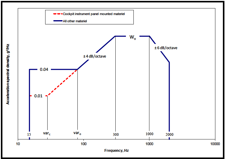
Figure description:
Acceleration spectral density vs Frequency
Legend
- Cockpit instrument panel mounted materiel — color: red; symbol: Dashed line with circular markers
- All other materiel — color: blue; symbol: Solid thick line
Annotations
- ± 4 dB/octave (text_label - position: Between frequency var_o and 300 Hz)
- W_o (text_label - position: Plateau between 300 Hz and 1000 Hz at level W_o)
- ± 6 dB/octave (text_label - position: Between frequency 1000 Hz and 2000 Hz)
| Frequency (Hz) | Cockpit instrument panel mounted materiel (g²/Hz) | All other materiel (g²/Hz) |
|---|---|---|
| 15 | null | 0.04 |
| var_c | 0.01 | null |
| var_o | 0.04 | 0.04 |
| 300 | W_o | W_o |
| 1000 | W_o | W_o |
| 2000 | null | null |
Notes: The x-axis is on a logarithmic scale. The values 'var_c', 'var_o', and 'W_o' are variables representing specific frequency and acceleration spectral density points defined by the profile. The 'Cockpit instrument panel mounted materiel' profile starts at (var_c, 0.01 and joins the 'All other materiel' profile at (var_o, 0.04.))
Figure 514.8D-1 - Category 12 - Fixed wing aircraft - jet aircraft. (Same as Annex C, Figure 514.8C-10.)
| W0 = WA + Σ1 n(WJ) W0, WA, WJ - Exposure levels in acceleration spectral density (g²/Hz). | |
|---|---|
| Aerodynamically induced vibration WA = a × b × c × (q)² | |
| Jet engine noise induced vibration WJ = {[0.48 × a × d × cos²(θ)/R] × [Dc × (Vc / Vr )³ + Df × (Vf / Vr )³]} | |
| a - Platform / Materiel interaction factor (see Annex A, paragraph 2.4). Note that this factor applies to Wo and not to the low frequency portion (15 Hz to break) of Figure 514.8D-1. = 1. 0 for materiel mounted on vibration isolators (shock mounts) and materiel weighing less than 36.3 kg. = 1. 0 ×10(0 6 - W / 60) for materiel weighing between 36.3 and 72.6 kg.(w = weight in kg) = 0. 25 for materiel weighing 72.6 kg or more. | Σ1 n - Jet noise contribution is the sum of the WJ values for each engine. |
| d - Afterburner factor. = 1. 0 for conditions where afterburner is not used or is not present. = 4. 0 for conditions where afterburner is used. | |
| b = Proportionality factor between vibration level and dynamic pressure (SI units). = 2.96 ×10⁻⁶ for materiel mounted on cockpit instrument panels. = 1.17 ×10⁻⁵ for cockpit materiel and materiel in compartments adjacent to external surfaces that are smooth and free from discontinuities. = 6.11 ×10⁻⁵ for materiel in compartments adjacent to or immediately aft of external surface discontinuities (cavities, chines, blade antennae, speed brakes, etc.), fuselage aft of wing trailing edge, wing, empennage, and pylons. | |
| R - Vector distance from center of engine exhaust plane to materiel center of gravity, m (ft). | |
| θ - Angle between R vector and engine exhaust vector (aft along engine exhaust centerline), degrees For 70 °< θ ≤ 180 ° use 70 °. | |
| c - Mach number correction. Note that this factor applies to W0 and not to the low frequency portion (15 Hz to varc or varo) of Figure 514.8D-1. = 1. 0 for 0 ≤ Mach ≤ 0. 9 = (-4.8M + 5.32) for 0.9 ≤ Mach ≤1. 0 (where M = Mach number) = 0.52 for Mach number greater than 1.0 | Dc - Engine core exhaust diameter, m (ft). |
| Df - Engine fan exhaust diameter, m (ft). | |
| Vr - Reference exhaust velocity, m/sec (ft/sec). = 564 m /sec (1850 ft/sec) | |
| q - Flight dynamic pressure, kN / m² (lb/ft²). | Vc - Engine core exhaust velocity (without afterburner, m/sec (ft/sec)) |
| Vf - Engine fan exhaust velocity (without afterburner, m/sec (ft/sec)) | |
| varc - intersection frequency for cockpit materiel based on 4dB/oct slope from W0 | |
| varo - intersection frequency for all other materiel based on 4dB/oct slope from W0 | |
| If Dimensions are in feet and pounds then: | |
| a = 1. 0 for materiel mounted on vibration isolators (shock mounts) and materiel weighing less than 80 lb. = 1. 0 ×10(0 60 - 0 0075 W) for materiel weighing between 80 and 160 lb. = 0. 25 for materiel weighing 160 lb. or more. | |
| b = 6.78 ×10⁻⁹, 2. 70 ×10-8, or 1.40 ×10⁻⁷ in the order listed above. | |
| Vr = 1850 feet / second | |
514.8-2.1 Basic Estimate Assumptions
Prediction estimates, measurement estimates, or a combination of prediction and measurement estimates may be considered in the same manner. It is assumed that uncertainty in individual measurements (processing error) does not affect the limit considerations. For measured field data digitally processed such that estimates of the SRS, ESD, FS, or ASD are obtained for single sample records, it is useful to examine and summarize the overall statistics of "similar" estimates selected in a way so as to not bias the summary statistics. To ensure the estimates are not biased, the measurement locations might be chosen randomly, consistent with the measurement objectives. Similar estimates may be defined as (1) estimates at a single location on materiel that has been obtained from repeated testing under essentially identical experimental conditions; (2) estimates on a system that have been obtained from one test, where the estimates are taken (a) at several neighboring locations displaying a degree of response homogeneity or (b) in "zones" i.e., points of similar response at varying locations; or (3) some combination of (1) and (2). In any case, it is assumed that there is a certain degree of homogeneity among the estimates across the frequency band of interest. This
MIL-STD-810H
METHOD 514.8, ANNEX F, APPENDIX B
latter assumption generally requires that (1) the set of estimates for a given frequency have no significant “outliers” that can cause large sample variance estimates, and (2) larger input stimulus to the system from which the measurements are taken implies larger estimate values.
514.8-2.1 File Setup (Step 1)
Step 1 is to define the test data of interest by selecting from the data files available on disk. The events selected should collectively represent the expected vibration exposure of the test item. It may be necessary to divide the events into groups of similar ASD shape and level, and produce LVTS separately for each group.
2.1.1 Effects of environment
Vibration results in dynamic deflections of and within materiel. These dynamic deflections and associated velocities and accelerations may cause or contribute to structural fatigue and mechanical wear of structures, assemblies, and parts. In addition, dynamic deflections may result in impacting of elements and/or disruption of function. Some typical symptoms of vibration-induced problems follow. This list is not intended to be all-inclusive:
- a. Chafed wiring.
- b. Loose fasteners/components.
- C. Intermittent electrical contacts.
- d. Electrical shorts.
- e. Deformed seals.
- f. Failed components.
- g. Optical or mechanical misalignment.
- h. Cracked and/or broken structures.
- i. Migration of particles and failed components.
- j. Particles and failed components lodged in circuitry or mechanisms.
MIL-STD-810H
METHOD 514.8
- k. Excessive electrical noise.
- Fretting corrosion in bearings.
514.8-2.1.1 Development test
Development testing is used to determine characteristics of materiel, to uncover design and construction deficiencies, and to evaluate corrective actions. Begin as early as practical in the development, and continue as the design matures. The ultimate purpose is to assure developed materiel is compatible with the environmental life cycle, and that formal testing does not result in failure. The tests have a variety of specific objectives. Therefore, allow considerable freedom in selecting test vibration levels, excitation, frequency ranges, and durations. Typical programs might include modal analysis to verify analytical mode shapes and frequencies, and sine dwell, swept sine, transient, or random vibration to evaluate function, fatigue life, or wear life. The test types, levels, and frequencies are selected to accomplish specific test objectives. Levels may be lower than life cycle environments to avoid damage to a prototype, higher to verify structural integrity, or raised in steps to evaluate performance variations and fragility.
514.8-2.1.1 Category 24 : All materiel - minimum integrity tests
Minimum Integrity Test (MIT) methods are generally relatively unsophisticated tests that can be adopted when a precise simulation is not necessary to establish suitability for service. These are normally coupled to generalized or fallback test severities that may be used in the earlier phases of a materiel development program when adequate information may not be available to allow use of project specific severities.
Note: Tailored test methods are preferred over MIT and should be employed whenever possible. MIT cannot be used for qualification.
The MIT test category is still employed and, therefore, continues to be included within the MIL-STD-810 guidelines; however, it is placed under the category “supplemental” due primarily to the unorthodox non-tailored nature of the test category with advice to implement with care.
The minimum integrity test is intended to provide reasonable assurance that materiel can withstand transportation and handling including field installation, removal, and repair. This is particularly important for materiel that was designed and tested to requirements based only on operational service environments in which the item is mounted on vibration isolators. The same hardware is often subjected to handling, transportation, etc., without isolators, and should be tested in such configurations. Subsequent to introduction of MIT in MIL-STD-810D, Environmental Stress Screening (ESS) has become a common practice in many production facilities. Generally, ESS testing is conducted at lower levels than those proposed in Figures 514.8E-1 and 514.8E-2, and spectral shaping based on structural characteristics of the materiel may be employed. Additionally, ESS testing is generally conducted in a hard mount configuration that may address the transportation test shortcomings addressed earlier in this paragraph pertaining to otherwise shock mounted equipment.
MIL-STD-810H METHOD 514.8, ANNEX E
Many agencies use some form of MIT based on historical knowledge of their particular service environments, and their spectra may vary from those provided within this document.
- a. Basis for levels. Vibration levels and durations of Figures 514.8E-1 and 514.8E-2 are not based on application environments. Rather, experience has shown that materiel that withstands these exposures functions satisfactorily in the field (unfortunately, much of the original documentation leading to the MIT levels was not carefully preserved). Since the MIT levels may be severe relative to most environments, failure to pass an MIT does not imply that the materiel will fail in its service environment. Failure to function subsequent to exposure to an MIT test should serve as grounds to make an attempt to define the test environment and make an effort at developing a tailored test.
- (1) Limitations. Do not apply minimum integrity tests to materiel that has been designed and tested to all environments of its life cycle, or to materiel that is otherwise tested to levels and durations that are equivalent to the minimum integrity test by the vibratory fatigue relationships of Annex A, paragraph 2.2. MIT cannot be used for qualification tests.
- (2) Delicate materiel. Use care with delicate materiel. Do not apply this test when the levels are felt to be too high for the materiel. Rather, evaluate the full environmental life cycle and make provisions to ensure the materiel is adequately protected from vibration and shock during all phases of the environmental life cycle - to include the transportation phase.
- (3) Exposure levels. Test levels are shown in Figure 514.8E-1 for general use, and in Figure 514.8E-2 for helicopter materiel. These exposures are to be applied directly to the materiel (hard mounted) and not through vibration isolation devices. These exposures are based on typical electronic boxes. When materiel is too large, unnecessarily high loads are induced in mounting and chassis structures, while higher frequency vibrations at subassemblies are too low. In these cases, apply the minimum integrity test to subassemblies. The maximum test weight of a materiel or subassembly should be approximately 36 kg (80 lb).
- (4) Exposure durations. Test durations are shown in Figure 514.8E-1 for general use, and in Figure 514.8E-2 for helicopter materiel.
In many cases, materiel is designed and tested to requirements based only on operational service environments. Other phases of the environmental life cycle are assumed to be less stringent or not considered. The minimum integrity test is intended to provide reasonable assurance that materiel can withstand transportation and handling including field installation, removal, and repair. This is particularly important for materiel mounted on vibration isolators in service and subjected to handling, transportation, etc., without isolators.
MIL-STD-810H METHOD 514.8, ANNEX E
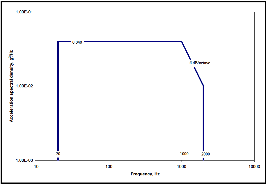
Figure description:
Annotations
- 0.040 (text_label - position: y = 0.040)
- -6 dB/octave (text_label - position: between 1000 Hz and 2000 Hz)
- 20 (vertical_line - position: x = 20)
- 1000 (vertical_line - position: x = 1000)
- 2000 (vertical_line - position: x = 2000)
| Frequency, Hz | Acceleration spectral density, g²/Hz |
|---|---|
| 20 | 0.040 |
| 1000 | 0.040 |
| 2000 | 0.010 |
Notes: The chart uses logarithmic scales for both the x-axis (Frequency, Hz and the y-axis (Acceleration spectral density, g²/Hz. The profile starts at 20 Hz, remains constant at 0.040 g²/Hz until 1000 Hz, and then slopes down at -6 dB/octave to 2000 Hz, reaching a value of 0.010 g²/Hz.))
Figure 514.8E-1. Category 24 - General minimum integrity exposure. (Test duration: One hour per axis; rms = 7.7 g's)
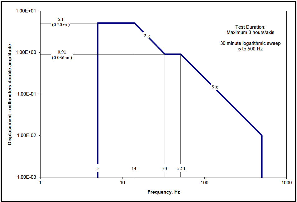
Figure description:
Displacement vs. Frequency Vibration Test Profile
Annotations
- 5.1 (0.20 in. (horizontal_line - position: y = 5.1))
- 0.91 (0.036 in. (horizontal_line - position: y = 0.91))
- 2 g (text_label - position: on slope between 14 Hz and 33 Hz)
- 5 g (text_label - position: on slope between 52.1 Hz and 500 Hz)
- Test Duration: Maximum 3 hours/axis (text_label - position: top right)
- 30 minute logarithmic sweep 5 to 500 Hz (text_label - position: top right)
| Frequency (Hz) | Displacement (mm double amplitude) |
|---|---|
| 5 | 5.1 |
| 14 | 5.1 |
| 33 | 0.91 |
| 52.1 | 0.91 |
| 500 | 0.01 |
Notes: The chart represents a vibration test profile with displacement measured in millimeters double amplitude versus frequency in Hz. The plot uses logarithmic scales for both axes. Vertical grid lines are marked at specific frequency transition points: 5, 14, 33, and 52.1 Hz.
Figure 514.8E-2. Category 24 - Helicopter minimum integrity exposure. (Test duration: Maximum three hours per axis – 30 minute logarithmic sweep 5 to 500 Hz.)
2.1.2 Sequence
Use the anticipated life cycle sequence of events as a general sequence guide (see Part One, paragraph 5.5).
- a. General. The accumulated effects of vibration-induced stress may affect materiel performance under other environmental conditions such as temperature, altitude, humidity, leakage, or electromagnetic interference (EMI/EMC). When evaluating the cumulative environmental effects of vibration and other environments, expose a single test item to all environmental conditions, with vibration testing generally performed first. If another environment (e.g., temperature cycling) is projected to produce damage that would make the materiel more susceptible to vibration, perform tests for that environment before vibration tests. For example, thermal cycles might initiate a fatigue crack that would grow under vibration or vice versa.
- b. Unique to this Method. Generally, expose the test item to the sequence of individual vibration tests that follow the sequence of the life cycle. For most tests, this can be varied if necessary to accommodate test facility schedules, or for other practical reasons. Complete all manufacture associated preconditioning (including ESS) before any of the vibration tests. Complete any maintenance associated preconditioning (including ESS) prior to tests representing mission environments. Perform tests representing critical end-of-mission environments last.
514.8-2.1.2 Qualification test
Qualification testing is conducted to determine compliance of a materiel with specific environmental requirements. Such tests are commonly a contractual requirement and will include specific test specifications. Qualification tests should be conducted using an excitation that has the same basic characteristics as the anticipated service environment. For most items, this consists of a functional test and an endurance test (sometimes combined). The functional test represents the worst case vibration (or envelope of worst case conditions) of the operational phases of the environmental life cycle. The endurance test is a fatigue test representing an entire life cycle. When separate functional and endurance tests are required, split the functional test duration, with one half accomplished before the endurance test, and one half after the endurance test (in each axis). The duration of each half should be sufficient to
MIL-STD-810H
METHOD
514.8-2.1.2 Category 25 - All vehicles - cantilevered external materiel
Material that consists of, or includes cantilever elements mounted external to a platform are subject to special problems. These problems are relatively rare but when they occur usually result in rapid and complete failure. These problems occur when the cantilevered elements are excited to vibrate in their cantilever bending or torsion modes by interaction with fluid flows.
- a. Excitation mechanisms. Cantilever elements immersed in a fluid flow can vibrate due to several types of self-excited vibration, and by forced response to pressure fluctuations. The three primary mechanisms are introduced below. For a general discussion of self-excited vibrations and more information on these three mechanisms, see paragraph 6.1, reference y, Chapter 7, and paragraph 6.1, reference z, paragraph 3.6, and chapters 5 and 6.
- (1) Flutter is a mechanism where the vibrations of a "wing" in a flow are such as to produce lift forces and moments that reinforce and amplify the vibration. A "wing" is a cantilever beam with slender cross section (i.e., the dimension parallel to the airflow is much larger than the dimension perpendicular to the flow). Flutter is not the result of an environmental forcing function. It is a mechanism inherent in a design and once started it needs no further environmental excitation to sustain and amplify the motion. Flutter is a separate engineering specialty and should be handled by flutter engineers. The vibration engineer needs to recognize flutter and the difference between flutter and other vibrations. Many artificial problems have been generated when other types of vibrations have been mislabeled as flutter. Conversely, flutter problems will not be solved until recognized as such and treated by flutter engineers.
- (a) A simple form is known as stall or stop sign flutter. Stop sign flutter can be seen when a plate
MIL-STD-810H METHOD 514.8, ANNEX E
(sign) mounted on a single central metal post flaps violently in the wind. This happens when the wind blows roughly parallel, but at a small angle to the vertical plane of the plate. A pressure distribution forms over the plate as with a "wing." These pressures combine as a lifting force located upstream (1/4 mean chord) of the post. This off center force causes the plate to twist the post, increasing the angle between the plate and the wind (angle of attack). Increased angle of attack causes increased lift, more twist of the post, and larger angle of attack. This continues until either the post torsional stiffness is sufficient to stop further twisting, or until the airflow over the plate stalls. When stall occurs, the center of lift shifts to the plate center (1/2 mean chord) and the twisting moment disappears. The post (torsional spring) returns the sign to the original angle, the flow reestablishes and the plate twists again, repeating the cycle. The cycle then repeats at the frequency of the plate/post torsion mode. With road signs this cycling can go on for long periods of time without failing the simple steel post. However, when a similar oscillation occurs with more sophisticated structures, failure usually occurs rapidly.
- (b) Classical flutter is a mechanism that involves two (or more) modes. Typically these are the first bending and first torsion modes. As flow speed increases the fluid interacts with the modal masses and stiffnesses, changing modal frequencies. Flutter occurs when modal frequencies converge and the motions of the two modes couple in a mechanism that extracts energy from the fluid flow. For additional information see paragraph 6.1, reference z, paragraph 7.10 or paragraph 3.6.
- (2) When air flows over a blunt cross section (depth ≈ height), vortices are shed alternately from one side, and then the other side, producing an oscillating force. These vortices are parallel to the length of the cantilever and propagate downstream as individual elements, dissipating rapidly. A blunt cross section cantilever attached to a platform moving through a fluid is subject to this force. When the excitation frequency is close to a cantilever resonant frequency, vibration will occur. When the vibrating mode is low, damped vibration can be substantial. This is another self-excited rather than an environment driven vibration. However, in this case, unlike flutter, the vibration engineer is usually expected to handle the problem.
(a) Vibration due to vortex shedding can often be seen in the radio antennae commonly used on automobiles (the single piece non-telescoping type). When moving at speeds of roughly 80 to 97 kilometers per hour (50 to 60 miles per hour) and when there is water on the antenna, the antenna often vibrates at easily visible amplitudes. It would appear that the antennae are not failing because the vibration is in the second bending mode (2 node points). The strain distribution (mode shape) is such (again clearly visible) that dynamic bending stresses are not very high at the root of the cantilever. (It is also suspected that the antennae are made of a low-strength steel that fortuitously has good fatigue properties.)
- (b) Shed frequency and force generated are approximately equal to:
f = 0.22 V/D
F = (1/2V DL)sin(2 ft)
f = frequency V = velocity D = cantilever cross section diameter F = force = density t = time L = the exposed length (perpendicular to the cross section)
(For non-circular cross sections, D becomes the dimension perpendicular to the flow in the frequency equation and the dimension parallel to the flow in the force equation. See paragraph 6.1, reference y, paragraph 7.6 for more information.)
- (3) Forced vibration of external cantilevers by fluctuations in a fluid flow is the same response to aerodynamic turbulence that is a primary source of vibration in aircraft. The factors that make this a special case for cantilevers are the dynamic characteristics of the cantilevers. First, a cantilever
MIL-STD-810H
exposes a large surface area to the excitation relative to the cross section of the support structure. Second, a cantilever tends to respond with high amplitude motion and large root stresses in the supporting base. Third, when the cantilever has the form of a "wing," aerodynamic lift and drag forces can be produced that add to the fluctuating pressure loads. These aerodynamic forces are produced because the turbulence is a tumbling of the fluid with variations in flow direction and flow velocity. These variations affect the "wing" as variations in angle of attack and flow velocity.
- (a) There are two types of excitation that are important. One is the broadband random turbulence behind any relatively blunt flow obstruction or behind a stalled airfoil. The other is vortices. A vortex forms when the pressures on two sides of a "wing" are different. The flow from the high pressure side wraps around the tip to the low pressure side. This results in a rotating flow trailing downstream of the tip. This rotating flow or vortex is left in the wake of the "wing," is highly stable, and persists for long distances downstream. Such a vortex is highly structured with a sharply peaked frequency distribution.
- (b) Vortex generators (small "wings") are often seen on airplane wings. The vortices generated help to hold the flow in the desired locations over the wing. This phenomenon can be clearly seen during takeoff of Boeing 737 aircraft equipped with CFM 56 (large diameter) engines when the air is humid. There is a vortex generator (small "wing") roughly 20 centimeters by 20 centimeters (8 inches by 8 inches) on the inboard side of each engine cowling. When the aircraft rotates to takeoff attitude, a vortex is formed that moves up over the wing and extends back parallel to the fuselage. Moisture condenses in the vortex, making it clearly visible to passengers seated at windows beside the engine and over the wing.
- b. Platform environments.
- (1) Fixed wing aircraft and external stores.
- (a) Any "wing" can flutter. However, this is not likely with blade antennas or the wings, control surfaces, and fins on stores. This is because first bending and first torsion mode frequencies are typically well separated. Any "wing" that has closely spaced bending and torsion mode frequencies should be evaluated by flutter engineers.
- (b) Fixed wing aircraft usually do not have blunt cross section external cantilevers. Anything outside the mold lines is generally streamlined (i.e., airfoil shaped) to reduce drag. However, if blunt cross sections are used, care should be exercised to ensure that shed frequencies and cantilever frequencies are well separated.
- (c) Many fixed wing aircraft have problems due to turbulence forced vibration. Typical problems are failed blade antennae, failed fins on external stores, and failed wings and control surfaces on missiles. Blade antenna problems are usually caused by locating the antenna downstream of a flow disturbance such as a cockpit canopy, a radome that projects into the air stream, or a cavity in the aircraft skin. Severe broadband flow turbulence carries downstream behind the disturbing element for a distance of three to five times the maximum cross sectional dimension of the disturbing element.
- (d) Fins on external stores are typically exposed to turbulence behind the carrying pylon, rack, or leading store. There is a case where a vortex forms in a corner of an engine inlet during high speed throttle chops. This vortex drops down and moves toward the airplane centerline as it extends aft. There is a single fuselage external store station that is wiped by this vortex. A specific missile carried at this station experienced high vibration levels of wings and control surfaces leading to rapid failure. The missile had to be redesigned to allow carriage on that one station.
- (2) Helicopters and external stores.
- (a) Flutter of "wings" on a helicopter is not likely due to the relatively low air speeds. However, if otherwise unexplainable failures occur in "wing" like elements, a flutter engineer should be consulted.
- (b) Flight speeds of helicopters are lower than fixed wing aircraft and streamlining is not as important. Thus, blunt cross section cantilevers are more likely to be used. When blunt cross sections are
MIL-STD-810H
used, care should be exercised to ensure that vortex shed frequencies and cantilever frequencies are well separated.
- (c) Helicopters are also subject to turbulence. However, turbulence produced vibratory loads are proportional to flow speed and helicopter speeds make problems due to turbulence relatively unlikely. It is still prudent to locate cantilevered materiel away from known turbulence.
- (3) Ground vehicles.
- (a) The flapping of the fabric cover of an open truck is a form of flutter. Structures of this type will "flutter" and must be strong enough and tied down well enough to prevent carrying away. However, to replace a fabric cover with a stiffened structure is not reasonable. Flutter problems at ground vehicle speeds should be limited to cases of this type.
- (b) Streamlining is usually not a significant factor in ground vehicle design. Thus, blunt cross-section cantilevers and vortex shedding are relatively likely. Exercise care to ensure vortex shed frequencies and cantilever frequencies are separated.
- (c) Forced vibration problems should be extremely rare due to low flow speeds. However, turbulence does exist at any flow speed and could possibly affect large, low frequency structures. The low frequency turbulence produced by large trucks affects the handling of smaller vehicles in close proximity. Vortices in the wakes of large trucks can often be seen in disturbances of roadside dust.
- (4) Watercraft.
- (a) For the portion of the platform above water, the discussion for ground vehicles applies. Portions of the platform below water are in a higher density fluid, even though flow speeds are low, the pressures are high. Wake turbulence of watercraft is clearly visible at the water surface. "Wing" materiel is subject to flutter and blunt cantilevers including "wing" elements with blunt trailing edges are subject to vortex shedding. Much of the original work in this technology dealt with watercraft problems.
- (b) Hulls and externally mounted underwater materiel are generally designed for smooth flow at the bow and along the sides but with squared off "boat tail" sterns. Turbulence driven forced vibration should not be a problem in smooth flow areas. However, anything located downstream of a "boat tail" will be subjected to high levels of flow turbulence.
c. Exposure levels
- (1) Exposure levels are not pertinent to flutter or other instabilities. These mechanisms, if they occur, will either drive the system to rapid, complete failure or will persist at high levels resulting in rapid fatigue or wear failure. The correct procedure is to design the materiel such that these mechanisms do not occur. When instabilities are discovered, the correct procedure is to understand and then eliminate the mechanism. This is accomplished by determining the mode shapes and frequencies of those resonances participating in the instability and, if possible, the characteristics of the flow field. Eliminating the mechanism is done by changing modal frequencies, mode shapes, modal damping, and/or flow characteristics. This is accomplished by changing modal mass, stiffness, or damping and/or by changing aerodynamic shapes. (See paragraph 6.1, reference z, paragraph 6.1.) Dynamic absorbers are often useful in changing modal properties (see paragraph 6.1, reference y, paragraphs 3.2 and 3.3).
- (2) Vortex shedding driven vibration also generally leads to rapid fatigue or wear failure. This problem typically involves a single mode of vibration of the materiel. If possible, the problem should be eliminated by separating the shed frequency and the resonant frequency (ideally by a factor of 2). If this is not practical, it may be possible to survive this mechanism for useful periods of time with good design. Good design consists of using materials with good fatigue properties, elimination of high stress points, and adding damping. In order to define exposure levels, it is necessary to measure the motions of the cantilever on the platform in the operating environment. These measurements are used to define modal responses. When laboratory tests are required, response control is necessary. This is
MIL-STD-810H
because the primary energy input is directly from the fluid flow. Response of the cantilever to this input is greater than the response to the vibration environment at the mount.
- (3) Local turbulence is not predictable except in a very general sense. Problems of this type should be avoided whenever possible by locating materiel away from known turbulence areas. Beyond this, it is necessary to operate the platform through its operational envelope and evaluate problems as they occur. When problems are discovered, the first approach should be to determine the source of the turbulent wake that is causing the problem and to move the materiel out of this wake. If this is not possible, proceed as discussed for vortex shedding problems.
- d. Exposure durations. As discussed above, problems should be solved by eliminating instability mechanisms or by moving materiel away from turbulence. If it is necessary to define exposure durations, take them from the LCEP. These problems may occur in very specific regions of an operating envelope. It may be necessary to break missions down to a very detailed level in order to define realistic durations.
Development of Laboratory Vibration Test Schedules
NOTE: Unless specifically noted, all document references refer to Annex F, Appendix F of this Method.
2.1.2.1 Functional test
Functional testing is conducted to verify that the materiel functions as required while exposed to no less than the worst case operational vibration for a particular segment(s) of a mission profile. Functional vibration levels typically do not include time compression but may include some level of conservatism. Tailor the vibration level for each segment of the mission profile based on measured data, when available, or derived from the operational state of the vehicle platform.. This is the maximum vibration environment where the unit under test is expected to function. Fully verify function at the beginning, middle and end of each test segment. Monitor basic function at all times during each test run. In some cases, materiel that must survive severe worst case environments may not be required to function or function at specification levels during worst case conditions. Typically "operating" and "non-operating" envelopes are established. Tailor functional tests to accommodate non-operating portions by modifying functional monitoring requirements as appropriate.
2.1.2.2 Endurance test
Endurance testing is conducted to reveal time-dependent failures. In many cases the test is accelerated in order to produce the same damage as the entire duration of the required service life. Generally, it is not required to have an item powered-up during the endurance phase of test. Refer to paragraph 2.1.2.1 for functional testing. Use the simplified fatigue relationship in paragraph 2.2 below to scale the less severe vibration levels to the maximum service levels that occur during the service life. This, in turn, will define the test time at maximum service levels (functional levels) that are equivalent to a vibration lifetime (levels vary throughout each mission). Use the equivalent time as the functional test duration, thereby combining functional and endurance tests. There may be cases when this test duration is too long to be compatible with program restraints. In these cases, use as long of a test duration as is practical and use the fatigue relationship to define the test level. While this approach does not completely eliminate nonlinearity questions, it does limit levels to more realistic maximums. Generally, the test item will not be in a powered-up state during the endurance (“non-operating”) phase of testing; particularly in a situation in which the test levels have been exaggerated beyond maximum measured values in order to significantly compress the test duration.
2.1.3 Durability test
Durability testing is a real-time (non-exaggerated) simulation of the environmental life cycle to a high degree of accuracy. A durability analysis precedes the test and is used to determine which environmental factors (vibration, temperature, altitude, humidity, etc.) must be included in the test to achieve realistic results. Although the test is intended to be a real time simulation of the life cycle, it may be shortened by truncation if feasible. Truncation is the elimination of time segments that are shown by the durability analysis to be benign with regard to materiel function and life. Durability analyses should use fatigue and fracture data applicable to each material, rather than the simplified expressions of paragraph 2.2 below.
- a. Worst case levels. Mission portions of the environmental life cycle are represented in the durability test by mission profiles. Mission profiles are statistical definitions of environmental stress and materiel duty cycle versus time. Mission profiles often do not include worst case environmental stresses because they are encountered too rarely to be significant statistically. However, it is important to verify that materiel will survive and function as needed during extreme conditions. Therefore, insert maximum environmental levels into the durability test, in a realistic manner. For example, in the case of a fighter airplane, the maximum levels would be inserted during an appropriate combat mission segment rather than a more benign segment such as cruise.
- b. Success criteria. Pass/fail criteria for durability tests are established for the particular effort. Criteria could include no failures, a maximum number of failures, a maximum amount of maintenance to fix failures, or some combination of these.
2.1.4 Reliability test
Reliability testing is accomplished to obtain statistical definitions of materiel failure rates. These tests may be development tests or qualification tests. The accuracy of the resulting data is improved by improving realism of the environmental simulation. Test requirements are developed by engineers responsible for materiel reliability. Specific definitions for reliability test as discussed in paragraph 6.1, reference aa, are provided below.
MIL-STD-810H
METHOD 514.8 ANNEX A
2.1.4.1 Statistical Reliability test
A statistical reliability test is a test performed on a large sample of production items for a long duration to establish or verify an assigned reliability objective for the equipment operating in its anticipated service environment, where the reliability objective is usually stated in terms of a mean-time-to-failure (MTTF), or if all failures are assumed to be statistically independent, a mean-time-between-failures (MTBF) or failure rate (the reciprocal of MTBF). To provide an accurate indication of reliability, such tests must simulate the equipment shock and vibration environments with great accuracy. In some cases, rather than applying stationary vibration at the measured or predicted maximum levels of the environment, even the non-stationary characteristics of the vibration are reproduced, often in combination with shocks and other environments anticipated during the service life (see Annex A of Method 516.8). The determination of reliability is accomplished by evaluating the times to individual failures, if any, by conventional statistical techniques.
2.1.4.2 Reliability Growth test
A reliability growth test is a test performed on one or a few prototype items at extreme test levels to quickly cause failures and, thus, identify weaknesses in materiel design. In many cases, the test level is increased in a stepwise manner to clearly identify the magnitude of the load needed to cause a specific type of failure. Design changes are then made and the failure rate of the materiel is monitored by either statistical reliability tests in the laboratory or valuations of failure data from service experience to verify that the design changes produced an improvement in reliability. Unlike statistical reliability tests, reliability growth tests do not simulate the magnitudes of the service environments, although some effort is often made to simulate the general characteristics of the environments; for example, random vibration would be used to test materiel exposed to a random vibration service environment.
2.1.5 Worthiness test
When unqualified materiel is to be evaluated in the field, verification that the materiel will function satisfactorily is normally required for safety and/or test efficiency reasons. This is accomplished by environmental worthiness test. The worthiness test is identical to a qualification test except that it covers only the life cycle of the field evaluation. Levels are usually typical operating levels unless safety is involved; then maximum operating levels are necessary. Durations are either equivalent to a complete system/subsystem test, long enough to check materiel function, or an arbitrary short time (5 or 10 minutes). For safety driven worthiness test, the test item is considered to be consumed by the test (the test item may not be used in the field). An identical item of hardware is used in the field evaluation. When safety is not an issue, an item may be subjected to a minimum time functional test and then used in the field evaluation. When it is required to evaluate the cumulative environmental effects of vibration and environments such as temperature, altitude, humidity, leakage, or EMI/EMC, a single test item should be exposed to all environmental conditions. For air worthiness testing, a three step approach may be required. For example, this could include conducting an initial laboratory vibration test, followed by experimental flight testing to acquire the actual exposure levels, and ending with a qualification test based on the measured field data.
2.1.6 Environmental Stress Screening (ESS)
ESS is not an environmental simulation test representative of a life cycle event and is not a substitute for a qualification test. It is a production or maintenance acceptance inspection technique designed to quickly induce failures due to latent defects that would otherwise occur later during service. However, it is an environmental life cycle event and should be included as preconditioning or as part of the test as appropriate. Materiel may be subject to multiple ESS cycles, and maintenance ESS vibration exposures may differ from production acceptance exposures. ESS should be included in development tests only as appropriate to the test goals. The vibration environment is sometimes applied using relatively inexpensive, mechanically or pneumatically driven vibration testing machines (often referred to as impact or repetitive shock machines) that allow little or no control over the spectrum of the excitation. Hence, the screening test environment generally does not represent an accurate simulation of the service environment for the materiel.
2.2 Selecting Procedures
Identify the environments of the materiel life cycle during the tailoring process as described in Part One, paragraph 4. Table 514.8-I provides a list of vibration environments by category versus test procedure. Descriptions of each category listed in this table are included in Annexes B - E, along with information for tailoring the test procedures of paragraph 4 below, and alternate test criteria for use when measured data are not available. In general, test the materiel for each category to which it will be exposed during an environmental life cycle. Tailor test procedures to best accomplish the test purpose (see Annex A, paragraph 2.1), and to be as realistic as possible (see Annexes B-E, paragraphs 1.2).
514.8-2.2 Test Time Compression and the Fatigue Relationship
The major cause of items failing to perform their intended function is material fatigue and wear accumulated over a time period as a result of vibration-induced stress. It is preferable for materiel to be tested in real-time so the effects of in-service conditions are simulated most effectively. However, in most instances real-time testing cannot be justified based on cost and/or schedule constraints and, therefore, it is customary to compress the service life environment into an equivalent laboratory test. For vibration environments that vary in severity during the materiel’s
MIL-STD-810H
METHOD 514.8 ANNEX A
service life, the duration of the environment can often be reduced for testing by scaling the less severe segments of the vibration environment to the maximum levels of the environment by use of an acceptable algorithm. In many cases, scaling less severe segments to the maximum levels may still yield a test duration that is still too long to be practical. In such cases, the same algorithm may be used to further reduce test duration by increasing test amplitude. Provided that fatigue is a significant potential failure criterion for the materiel under test, this practice is acceptable within strict limits, notably that test amplitudes are not over exaggerated (or accelerated) simply to achieve short test durations. Such excessive amplitudes may lead to wholly unrepresentative failures, and cause suppliers to design materiel to withstand arbitrary tests rather than the in-service conditions.
The most commonly used method for calculating a reduction in test duration is the Miner-Palmgren hypothesis that uses a fatigue-based power law relationship to relate exposure time and amplitude. The mathematical expression and variable descriptions for this technique are illustrated below in Equations (1) and (4).
12 S₁ = Equation (1) t₁
where
t1 = equivalent test time
t2 = in-service time for specified condition
S1 = severity (rms) at test condition
S2 = severity (rms) at in-service condition
[The ratio is commonly known as the exaggeration factor.]
m = a value based on (but not equal to) the slope of the S-N curve for the appropriate material, where S represents the stress amplitude, and N represents the mean number of constant amplitude load applications expected to cause failure.
Fatigue damage can be calculated using either a stress life or strain life process. For the strain life technique, the number of cycles to failure, N , is computed from: f
σ' E = = (2N₁ ) + ɛ', (2 N₁ ) Equation (2) E
where
where = test or environment strain amplitude = fatigue strength coefficient (material property) = modulus of elasticity (material property) = number of cycles to failure = fatigue strength exponent (material property) = fatigue ductility coefficient (material property) = fatigue ductility exponent (material property)
The fatigue strength portion of the equation represents the elastic portion of the S-N curve and the fatigue ductility portion of the equation represents the plastic portion. The stress life technique uses only the linear (elastic) portion of the curve (below yield) and is written as:
S₁ =σ', (2N) Equation (3)
where
test or environment stress amplitude
Equation (3) is valid only in the finite life region with elastic nominal stresses (generally 1000 to 10,000,000 cycles
MIL-STD-810H
METHOD
514.8-2.2 Category 2 - Shipping and Handling
Parts, subassemblies, and materiel are subject to vibration during handling and transportation within and between manufacturing and maintenance facilities. When there are significant differences between exposures to different serial number items (lots), select vibration test articles from those lots that experience the maximum vibration exposure, and determine exposure durations from manufacturing and maintenance planning. Where transportation is by normal commercial means, use the applicable guidance of Annex C, paragraph 2. For other means of transportation, measure exposure levels.
514.8-2.2 Category 5 - Truck/trailer - loose cargo
The cargo has freedom to bounce, scuff and collide with other cargo and with the sides of the vehicle. The loose cargo environment includes conditions experienced by cargo transported in a vehicle traversing irregular surfaces. This test replicates the repetitive random shock environment incurred by cargo transported under these conditions. This test does not address general cargo deck vibration or individual shocks or impacts inflicted during handling or accidents.
- a. Test bed. (See Figure 514.8C-8.) Cover the test bed of the package tester with a cold rolled steel plate (see note below), 5 to 10 mm (0.2 to 0.4 in) thick, and secure the plate with bolts. The tops of the heads should be slightly below the surface. Space the bolts at sufficient intervals around the four edges and through the center area to prevent diaphragming of the steel plate. Do not start a test on an area of steel plate that is severely damaged or worn through.
Note: Comparison of plywood bed and steel bed data show no statistical difference. Also, steel beds require less maintenance and US Army trucks use steel beds. See paragraph 6.1, reference a.
- b. Fencing. Two different setups of fencing are required depending on the type of test item. The two types are those that are more likely to slide on the test surface or “rectangular cross section items” (typically packaged items), and those most likely to roll on the surface, or “circular cross section items.” ("Multiple test items" refers to identical test items, and not to a mixture of unrelated test items.) The fence opposite the vertical impact wall is not intended as an impact surface, but is used to restrain the test item from leaving the tester. The distance to this restraining fence should be sufficient to prevent constant impact, but still prevent one or more of multiple test items from “walking” away from the others. The height of the test enclosure (sideboards, impact wall, and restraining fence) should be at least 5 cm higher than the height of the test item to prevent unrealistic impacting of the test item on the top of the enclosure.
- c. Test item structure.
- (1) Materiel likely to slide (e.g., flat-bottomed). Using suitable fixturing as described previously, the test item is placed on the test machine. The wooden impact walls are configured so as to allow impacting on only one end wall (no rebounding), and to prevent unlimited rotation of test items that are non-symmetrical about the vertical axis. Multiple test items are not separated from one another by sideboards. The test item is positioned in its most likely transport orientation. In the event the most likely transport orientation cannot be determined, the test item is placed on the bed with the longest axis horizontal and parallel to the plane of rotation of the bed. The default space around the perimeter of a test item or an item and a barrier wall is a minimum of one inch (25.4 cm) at the start of testing. The spacing varies during testing and is not controlled. After one-half the total designated test time, stop the test, reposition the test item to an alternate orientation, and continue the test.
- (2) Materiel likely to roll (e.g., circular cross section). For the circular cross section items, place the impact walls and sideboards so as to form a square test area. The size of the test area is determined by a series of equations presented below. Sw and SB are chosen based on test item geometry to provide realistic impacting with the test bed impact walls and between test items. A typical value for both Sw and SB is 25 mm. Use the following formulae to determine the test area dimension:
For values of the number of test items, N > 3, compute the required slenderness ratio, Rr, from Equation (1):
Equation (1)
| Symbol | Definition | Section |
|---|---|---|
| required slenderness ratio | ||
| length of the test item, cm | ||
| diameter of the test item, cm | ||
| number of test items | ||
| space between test item and wall, cm | ||
| space between each test item, cm Compute the test item actual slenderness ratio, , from |
Ra=L/D Equation (2) and it is independent of the number of test items, N. If the actual test item slenderness ratio, Ra, is greater than the required ratio, R₂, computed in Equation (1), then: X=0.767 L√N Equation (3)
X= length of each side of the square test area
If the actual test item slenderness ratio, Ra, is less than the required ratio, R₁, computed in Equation
(1), then:
X = ND +2Sw+(N−1)SB Equation (4)
For values of N ≤3, the required slenderness ratio, R₁, is computed from Equation (5):
NL R₁ = Equation (5) 1.5L-2S-(N-1)SB
If the actual test item slenderness ratio, Ra, is greater than the required ratio, R₂, computed in Equation (5), then: X≥ 1.5L Equation (6)
Otherwise:
X is computed from Equation (3).
Generally, if the actual slenderness ratio, L/D, is greater than 4, Equations (3) or (6), (depending upon the number of test items) are applicable.
- d. Test item placement. For either type test item, the materiel is placed on the test machine in a non-uniform manner. Because part of the damage incurred during testing of these rolling items is due to them impacting with each other, the number of test items should be greater than three. After the designated test time, stop the test.
- e. Exposure levels. This environment is a function of package geometry and inertial properties, vehicle geometry, and the complex vibratory motion of the vehicle cargo bed. No database exists for input vibration to simulate this environment. However, the test discussed below will provide a generally conservative simulation of the environment.
- (1) Two methodology studies (paragraph 6.1 references g and h) determined that Figure 514.8C-8 package test equipment, operated in circular synchronous mode, provides a reasonable loose cargo simulation.
The equipment motion required is a 2.54 cm (1.0 inch) diameter orbital path at 5 Hz (300 RPM, approximately 1.3 g). Test equipment should have the capability to maintain the speed at 300 ±2 RPM. Tables operated near maximum load capacity or with an unbalanced test item(s) may require a larger RPM tolerance. The use of a package tester operating in non-synchronous, vertical linear motion, or a single axis vibration system, is not an acceptable substitute for the loose cargo test requirement.
- (2) This test is not tailorable and cannot be directly interpreted in terms of materiel design requirements.
- f. Exposure durations. A duration of 20 minutes represents 240 km (150 miles) of transportation (encompassing truck, two-wheeled trailer, and tracked vehicle), over the various road profiles found in the transport scenario from the Corps Staging Area to a Using Unit (see Figure 514.8C-1). Use ratio scenario times in the materiel Life Cycle Environment Profile to define exposure times.
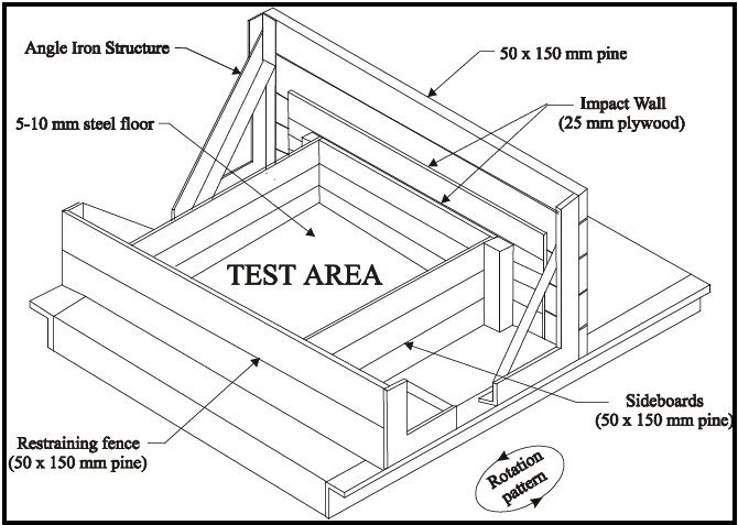
Figure description:
Figure 514.8C-8: Category 5 - Loose cargo test setup
- Test Area: Central compartment with a 5-10 mm steel floor.
- Impact Wall: Constructed from 25 mm plywood.
- Enclosure Materials:
- Restraining fence: 50 x 150 mm pine.
- Sideboards: 50 x 150 mm pine.
- Top rails: 50 x 150 mm pine.
- Support Structure: Backed by an angle iron structure.
- Movement: Designated rotation pattern indicated at the base.
Figure 514.8C-8. Category 5 - Loose cargo test setup.
514.8-2.2 Category 13 - Propeller aircraft
The vibration environment for materiel installed in propeller aircraft (except engine-mounted, see paragraph 2.11, and gunfire induced (see Method 519.8)) is primarily propeller induced. The vibration frequency spectra consists of a broadband background with superimposed spikes (see paragraph 6.1, references n through t). The spikes are more nearly sinusoidal than narrowband and are best represented utilizing sine-on-random vibration. The background spectrum results from various random sources (see paragraph 2.1) combined with many lower level periodic components due to the rotating elements (engines, gearboxes, shafts, etc.) associated with turboprops. The spikes are produced by the passage of pressure fields rotating with the propeller blades. These occur in relatively narrow bands centered on the propeller passage frequency (number of blades multiplied by the propeller rpm) and harmonics.
- a. Constant propeller speed. Most current propeller aircraft are constant-speed machines. This means that rpm is held constant and power changes are made through fuel flow changes and variable-pitch blades, vanes, and propellers. These machines produce fixed frequency spikes like those of Figures 514.8D-2 at the blade passing frequency and harmonics.
- b. Varying propeller speed. When propeller speed varies during operation, the frequency of the spikes change. This can be represented by swept sine tests with the sweep bandwidths encompassing the propeller speed variations of operation. Separate spectra may be required to describe individual mission segments.
- c. Source dwell testing. These vibration environments can be approximated in the laboratory by the source dwell test described in Annex A, paragraph 2.3.3. Vibration problems in this type of environment are typically associated with the coincidence of materiel vibration modes and excitation spikes. Intelligent designs use notches between spikes as safe regions for materiel vibration modes. It is particularly important to assure that vibration isolation frequencies do not coincide with spike frequencies. Source dwell tests minimize the likelihood that materiel will be overstressed at non-representative conditions, and ensure reasonable design provisions will not be subverted.
- d. Exposure levels. Whenever possible, use flight vibration measurements to develop vibration criteria. When measured data are not available, endurance levels can be derived from Table 514.8D-II, and Figures 514.8D-2 and 514.8D-3. Functional test levels can be derived by scaling the endurance ASD levels (broadband and L0) by a factor of 0.35. Reliability test levels can be derived by scaling the endurance levels by a factor of 0.22. Once scaled L0 can be converted to an equivalent sine tone (S0) using the formula provided in Table 514.8D-II. Subsequent harmonics (S1, S2, and S3, corresponding to f1, f2, and f3) are calculated from S0 dropping 3 dB in amplitude per octave. Tests should be conducted as sine-on-random vibration, with sine levels calculated as defined in Table 514.8D-II and Figure 514.8D-2.
- e. Exposure durations. Take durations from the Life Cycle Environment Profile. If LCEP data are not available for development of the test durations, endurance tests should be conducted for one hour per axis which equivalent to 1000 hours of flight. Test durations associated with functional testing should be kept to a minimum and it is generally not considered part of the endurance test duration. Test duration for reliability testing should be set to the total flight hours required, divided equally among the three test axes, and can be considered as part of the endurance test. For equipment that will be installed on multiple fixed wing propeller aircraft the test can be divided equally between all aircraft types.
MIL-STD-810H
METHOD 514.8, ANNEX D
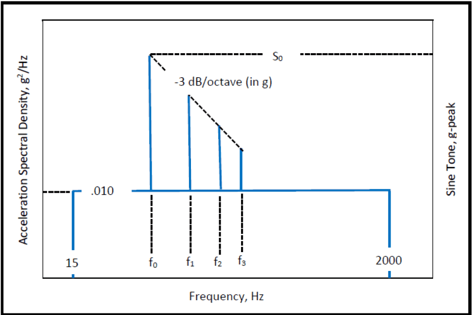
Figure description:
Combined Random and Sine Vibration Environment Profile
Acceleration Spectral Density and Sine Tone vs. Frequency
Annotations
- -3 dB/octave (in g (slope_line - position: Dashed line starting from the peak of the sine tone at f₀ (level S₀ and passing through peaks at f₁, f₂, and f₃.)))
- S₀ (horizontal_line - position: y = S₀ on the Sine Tone, g-peak axis.)
- .010 (horizontal_line - position: y = 0.010 on the Acceleration Spectral Density, g²/Hz axis.)
| Frequency, Hz | Acceleration Spectral Density, g²/Hz | Sine Tone, g-peak |
|---|---|---|
| 15 | 0.010 | null |
| f₀ | 0.010 | S₀ |
| f₁ | 0.010 | peak on -3 dB/octave slope |
| f₂ | 0.010 | peak on -3 dB/octave slope |
| f₃ | 0.010 | peak on -3 dB/octave slope |
| 2000 | 0.010 | null |
Notes: The graph depicts a constant Acceleration Spectral Density (ASD of 0.010 g²/Hz between 15 Hz and 2000 Hz. Discrete sine tones are shown at specific frequencies f₀, f₁, f₂, and f₃. The sine tone at f₀ has a peak value of S₀. The peak values of subsequent sine tones at f₁, f₂, and f₃ follow a downward slope of -3 dB/octave relative to the peak at f₀.)
Figure 514.8D-2. Category 13 - Propeller aircraft vibration exposure.
| TRANSPORTATION LOCATIONS (see Figure 514.8D-3) | NARROWBAND LEVEL L0 (g2/Hz) |
|---|---|
| In fuselage or wing forward of propeller | 0.1 |
| Within one propeller blade radius of propeller passage plane | 1.2 |
| In fuselage or wing aft of propeller | 0.3 |
| In engine compartment, empennage, or pylons | 0.6 |
| 1/ For Materiel mounted to external skin, increase level by 3 dB. | |
| 2/ f0 = blade passage frequency (propeller rpm times number of blades) (Hz). f1 = 2 × f0 f2 = 3 × f0 f3 = 4 × f0 | |
| 3/ Test should be conducted as sine-on-random, with: S0 = 1.414 * √(0.1 * f0 * L0) | |
| 4/ Sine tones may be swept to account for known variance in blade passing frequency. | |
| 5/ C-130 Aircraft: 4 blade propeller - f0 = 68 Hz (C-130K); 6 blade propeller - f0 = 102 Hz (C-130J) | |
| 6/ Endurance test duration per axis: 1 hour for 1000 hours of flight. | |
MIL-STD-810H METHOD 514.8, ANNEX D
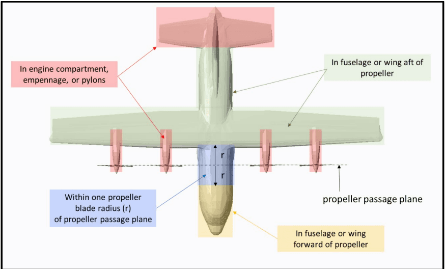
Figure description:
- Document Source: MIL-STD-810H, Method 514.8, Annex D
- Subject: Category 13 - Propeller aircraft installed equipment locations
- Key Entities & Zones:
- Propeller Passage Plane: Defined by a dashed horizontal line intersecting the propeller hubs.
- Within one propeller blade radius (r of propeller passage plane: Highlighted in blue, centered on the passage plane along the fuselage.
- In engine compartment, empennage, or pylons: Highlighted in red; covers the tail section and the four engine nacelle/pylon areas.
- In fuselage or wing aft of propeller: Highlighted in green; covers the main wing structure and the fuselage section behind the propeller passage plane.
- In fuselage or wing forward of propeller: Highlighted in yellow; covers the nose/cockpit section of the fuselage forward of the blue zone.
Figure 514.8D-3. Category 13 - Propeller aircraft installed equipment locations.
514.8-2.2 Basic Estimate Summary Preprocessing
There are two ways in which summaries may be obtained. The first way is to use an "enveloping" scheme on the basic estimates to arrive at a conservative estimate of the environment, and some qualitative estimate of the spread of basic estimates relative to this envelope. This procedure is dependent upon the judgment of the analyst and, in general, does not provide consistent results among analysts. The second way is to combine the basic estimates in some statistically appropriate way and infer the statistical significance of the estimates based upon probability distribution theory. Reference g summarizes the current state of knowledge relative to this approach and its relationship to determining upper limits on sets of data. In general, the estimates referred to and their statistics are related to the same frequency band over which the processing takes place. Unfortunately, for a given frequency band, the statistics behind the overall set of estimates are not easily accessible because of the unknown distribution function of amplitudes for the frequency band of interest. In most cases the distribution function can be assumed to be normal, provided the individual estimates are transformed to a "normalizing" form by computing the logarithm to the base ten of the estimates. For ESD and FS estimates, the averaging of adjacent components (assumed to be statistically independent) increases the number of degrees of freedom in the estimates while decreasing the frequency resolution with the possible introduction of statistical bias in the estimates. For ASD estimates, averaging of adjacent components can be useful provided the bias error in the estimate is small; i.e., the resolution filter bandwidth is a very small fraction of the overall estimate bandwidth. For SRS estimates, because they are based on maximum response of a single- degree-of-freedom system as its natural frequency is varied, adjacent estimates tend to be statistically dependent and, therefore, not well smoothed by averaging unless the SRS is computed for very narrow frequency spacing. In such cases, smoothing of SRS estimates is better accomplished by reprocessing the original time history data at a broader natural frequency spacing, e.g., 1/6th octave as opposed to 1/12th octave. There is no apparent way to smooth dependent SRS estimates mathematically when reprocessing cannot be performed, and the acceptable alternative is some form of enveloping of the estimates. The larger the sample size, the closer the logarithm transform of the estimates is to the normal distribution unless there is a measurement selection bias error in the experiment. Finally, generally, before application, the upper limits obtained in the paragraphs to follow are smoothed by straight line segments intersecting at spectrum “breakpoints.” No guidance is provided in this appendix relative to this “smoothing” or “enveloping” procedure, e.g., whether estimates should be clipped or enveloped and the relationship of the bandwidth of the estimates to the degree of clipping, etc., except that such smoothing should be performed only by an experienced analyst. Reference g discusses this further.
514.8-2.2 Select Event Start and End Time (Step 2)
During the collection of the raw field data, it is common practice to begin acquisition prior to reaching a desired speed or start of a particular road surface or maneuver. For this reason, the analyst may need to select only a portion of the digitized data set provided for a particular event. It is helpful to define the start and end time of the data set to be carried forward in the VSD process.
MIL-STD-810H
METHOD 514.8, ANNEX F, APPENDIX D
2.2.1 Procedure selection considerations
Vibration test profiles may be omitted from an overall test series depending on relative profile severity. Profile severity comparisons shall include fatigue damage potential (test duration and bandwidth), vibration amplitude, and spectral content within the profile bandwidth. Analytical estimates of fatigue damage potential should be made on the basis of simple, well-understood models of the materiel, when and if possible.
Another method for reducing test duration is through a combination of spectra techniques. Combinations of random vibration test profiles may be performed if the reference spectra and bandwidths are similar by either employing the fatigue damage spectrum (FDS) or via statistical methods (refer to Annex F). Combination of vibration tests should not be performed with dissimilar spectra or spectra with dissimilar bandwidths. Examples of dissimilar spectra are random, sine, sine on random, sweeping sine on random, or sweeping random on random. For example, combining a broadband random (e.g. wheeled vehicle) spectrum with a sine-on-random spectrum (e.g. helicopter) should be avoided. Observe that the FDS example provided in Annex F is quite liberal in combining spectral shapes. Factors such as vibration magnitudes and unit under test (UUT) robustness should always be considered in establishing combined spectra based requirements.
Extreme caution should be used if test schedule compression is used to combine tests. Too much compression could result in entering non-linear regions of mechanical response which is undesirable. Highly conservative specifications with no correlation to actual discrete environmental conditions can lead to unnecessary overdesign. Furthermore, combining spectra can result in the inability to relate a failure mechanism to a discrete vibration environment. Finally, careless combination of spectra has the potential to yield a test that is difficult to conduct and control. Additionally, enveloping or combining spectra could result in the loss of vehicle anti-resonances which may be necessary for laboratory replication. These considerations are especially important for multi-axis test setups and profile definitions.
In evaluation of the relative severity of environments, include the differences in transportation configuration (packaging, shoring, folding, etc.) and application configuration (mounted to platform, all parts deployed for service,
MIL-STD-810H
METHOD 514.8
etc.). In addition, transportation environments are usually defined as inputs to the packaging, whereas application environments are expressed as inputs to the materiel mounting structure or as response of the materiel to the environment.
- a. Transportation vibration more severe than application environment. Transportation vibration levels are often more severe than application vibration levels for ground-based and some shipboard materiel. In this case, both transportation and platform vibration tests are usually needed because the transportation test is performed with the test item non-operating, and the platform test is performed with the test item operating.
- b. Application vibration more severe than transportation vibration. If the application vibration levels are more severe than the transportation levels, it may be feasible to delete transportation testing. It may also be feasible to change the application test spectrum shape or duration to include transportation requirements in a single test. In aircraft applications, a minimum integrity test (see Annex E, paragraph 2.1) is sometimes substituted for transportation and maintenance vibration requirements.
- c. Any omission or combination of spectra techniques employed should be agreed to by the responsible test authority prior to the conduct of testing and should be thoroughly documented in the test report.
2.2.2 Difference among procedures
- a. Procedure I - General Vibration. Use Procedure I for materiel to be transported as secured cargo or deployed for use on a vehicle. This procedure applies to ground vehicles as well as fixed and rotary wing aircraft. For this procedure, the test item is secured to a vibration exciter, and vibration is applied to the test item as an input at the fixture/test item interface. Steady state or transient vibration may be applied as appropriate.
- b. Procedure II - Loose Cargo Transportation. Use this procedure for materiel to be carried in/on trucks, trailers, or tracked vehicles and not secured to (tied down in) the carrying vehicle. The test severity is not tailorable, and represents loose cargo transport in military vehicles traversing rough terrain.
- c. Procedure III - Large Assembly Transportation. This procedure is intended to replicate the vibration and shock environment incurred by large assemblies of materiel installed or transported by wheeled or tracked vehicles. It is applicable to large assemblies or groupings forming a high proportion of vehicle mass, and to materiel forming an integral part of the vehicle. In this procedure, use the specified vehicle type to provide the mechanical excitation to the test materiel. The vehicle is driven over surfaces representative of service conditions, resulting in realistic simulation of both the vibration environment and the dynamic response of the test materiel to the environment. Generally, measured vibration data are not used to define this test. However, measured data are often acquired during this test to verify that vibration and shock criteria for materiel subassemblies are realistic.
- d. Procedure IV - Assembled Aircraft Store Captive Carriage and Free Flight. Apply Procedure IV to fixed wing aircraft carriage and free flight portions of the environmental life cycles of all aircraft stores, and to the free flight phases of ground or sea-launched missiles. Use Procedure I, II, or III for other portions of the store’s life cycle as applicable. Steady state or transient vibration may be applied as appropriate. Do not apply Procedure I to fixed wing aircraft carriage or free flight phases.
2.3 Determine Test Levels and Conditions
Select excitation form (steady state or transient), excitation levels, control strategies, durations and laboratory conditions to simulate the vibration exposures of the environmental life cycle as accurately as possible. Whenever possible, acquire measured data as a basis for these parameters. Annexes B - E include descriptions of various phases typical of an environmental life cycle, along with discussions of important parameters and guidance for developing test parameters. Annex A has further guidance in interpretation of technical detail.
514.8-2.3 Vibration Characterization
The majority of vibration experienced by materiel in operational service is broadband in spectral content. That is, vibration is present at all frequencies over a relatively wide frequency range at varying intensities. Vibration amplitudes may vary randomly, periodically, or as a combination of mixed random and periodic.
MIL-STD-810H METHOD
514.8-2.3 Category 3 - Environmental Stress Screening (ESS)
Parts, subassemblies, and materiel are often subject to ESS vibration exposures during manufacturing and maintenance. While exposure levels are identical for each like item, exposure durations are not. Items can be subjected to multiple cycles of ESS prior to production acceptance. Further, exposures are often significant with respect to vibratory fatigue. Include maximum allowable exposures in design calculations and as environmental test preconditioning. Use specified exposure levels and the maximum allowable production and maintenance exposure durations for part, subassembly, and materiel ESS.
Downloaded from https://www.everyspec.com
MIL-STD-810H METHOD 514.8, ANNEX B
(This page is intentionally blank.)
MIL-STD-810H METHOD 514.8, ANNEX C
METHOD 514.8, ANNEX C Transportation Tailoring Guidance for Vibration Exposure Definition
NOTE: Unless specifically noted, all document references refer to paragraph 6.1 of the front part of this Method.
514.8-2.3 Category 6 - Truck/trailer - large assembly transport
For large materiel, it is necessary to recognize that the materiel and the transport vehicle vibrate as a flexible system (see Annex A, paragraph 2.4). In such cases, transportation conditions may be simulated using the actual transport vehicle as the vibration exciter. The test assemblage may consist of materiel mounted in a truck or trailer, or materiel mounted in a shelter that is then mounted on a truck, trailer, or dolly set. Ensure the materiel is mounted and secured on the transport vehicle(s) that is used during actual transport. Provide instrumentation to measure vertical vibration of the materiel mounts, cargo floor, or shelter floor. Provide additional instrumentation as needed to determine the vibration of the materiel and critical subassemblies.
Note: This procedure is suitable for measuring or testing for the transportation or ground mobile environment of materiel of any size or weight. For smaller cargo loads, the assemblage should be either the specific design cargo load or the most critical cargo load(s) for the transport vehicle as appropriate.
- a. Exposure levels. The assemblage should be in its deployment configuration and mounted on the vehicle for which it was designed. If the assemblage is to be contained in a shelter, it should be installed within the shelter in the deployment configuration. The exposure consists of traversing the transport vehicle over a prepared test course. The test course and vehicle speeds should represent the transportation terrain/road conditions of the LCEP. Transport vehicle speeds may be limited either by the vehicle's safe operating speed over a specific course profile, or by the speed limit set for the specific course. An example based on test surfaces available at the US Army Aberdeen Test Center (paragraph 6.1, reference b) is as follows. Drive the test vehicle over each of the following test surfaces. Operate at the specified speeds unless these exceed safe driving conditions. In this case, define and coordinate maximum safe operating speeds with
MIL-STD-810H
METHOD 514.8, ANNEX C
the authority responsible for the environmental requirements.
| Vehicle Speed km/hr (mph) | Course Length m (ft) | ||||
|---|---|---|---|---|---|
| (1) | Coarse washboard [150 mm (6 in) waves; 1.8 m (6 ft) apart] | 8 | (5) | 243 | (798) |
| (2) | Belgian block | 32 | (20) | 1201 | (3940) |
| (3) | Radial washboard [50 mm (2 in) to 100 mm (4 in) waves] | 24 | (15) | 74 | (243) |
| (4) | Two inch washboard [50 mm (2 in) waves, 0.6 m (2 ft) apart] | 16 | (10) | 251 | (822) |
| (5) | Three inch spaced bump [75 mm (3 in) bumps] | 32 | (20) | 233 | (764) |
- b. Exposure durations. Ensure the durations (distances) of each test course segment/speed combination are in accordance with the scenario(s) of the Life Cycle Environment Profile. If the LCEP in-service road information is not available, the minimum test duration is defined by operation of the vehicle five individual times on the full length of each test course above, or an equal total distance at the indicated or test plan defined speed(s).
514.8-2.3 Category 14 - Rotary wing aircraft - helicopter
Helicopter vibration (for engine-mounted materiel, see paragraph 2.11 below, and for gunfire induced vibration, see Method 519.8) is characterized by dominant peaks superimposed on a broadband background, as depicted in Figure 514.8D-4. The peaks are sinusoids produced by the major rotating components (main rotor, tail rotor, engine, gearboxes, shafting, etc.). The peaks occur at the rotation speed (frequency) of each component (i.e., 1P for main rotor, 1T for tail rotor, and 1S where S designates a locally predominate rotating element) and harmonics of these speeds (e.g., 2P, 3P, 4P). The broadband background is a mixture of lower amplitude sinusoids and random vibrations due to sources such as aerodynamic flow noise (see paragraph 2.1). Vibration levels and spectrum shapes vary widely between helicopter types and throughout each helicopter, depending on strength and location of sources and the geometry and stiffness of the structure. Thus, the need for measured data is acute.
- a. Broadband background. The broadband background is expressed as random vibration for design and test purposes as a matter of expediency. The definition of and application to design and test of all lower level sinusoidal and random components is not practical.
- b. Dominant sinusoids. The dominant sinusoids are generated by rotating components of the helicopter, primarily the main rotor(s), but also tail rotor, engine(s), drive shafts, and gear meshing. The normal operating speeds of these components are generally constant, varying less than five percent. However, recent designs have taken advantage of variable rotor speed control that generates a pseudo steady state rotor speed at values between 95 and 110 per cent of the nominal rotor speed. This complicates the materiel design and test process since all rotating component speeds, pseudo or otherwise, should be accounted for.
- c. Variable rotor speeds. Variable speed helicopters are also possible; in this case they also account for the full range of rotation speeds. A range of 0.975 times minimum speed to 1.025 times maximum speed is recommended.
- d. Design practice. An obvious requirement for helicopter materiel design is to avoid a match or near match between materiel resonant frequencies and the dominant sinusoids. A minimum clearance between operating speed and resonant frequency of at least five percent is recommended. It is important to note that helicopter frequencies and amplitudes are unique for each helicopter type and, to some degree, each model of a given type.
e. Exposure levels
- (1) For reasons stated above, the exposure levels for materiel installed in helicopters should be derived from field measurement (additional tailored helicopter vibration schedules are provided in paragraph 6.1, reference xx). When measured data are not available, levels can be derived from Table 514.8D-III, and Figures 514.8D-4 and 514.8D-5.
NOTE: These levels are intended to envelope potential worst-case environments, and have been aggressively compressed in time (paragraph 6.1, reference ww indicates a time compression from 2500 hours to 4 hours using the equation shown in paragraph 2.3f with a value of m=6). They do not represent environments under which vibration-sensitive materiel should be expected to perform to specification. However, the materiel is expected to survive undamaged, and to function to specification at the completion of the test. Functional test levels can be derived as discussed below in paragraph 2.3e (4).
Materiel costs are often strongly influenced by the performance required in a vibration environment. Consequently, field measurement based vibration criteria can be very important and are strongly recommended.
Data acquired from variants of the rotorcraft listed in Table 514.8D-IIIa, were used to develop the random levels, source frequency relationships, and peak acceleration relationships reported in Table 514.8D-IIIb. Aircraft specific source frequencies are directly associated with rotor blade count and rotation speed. Tabulated source frequency ranges, peak acceleration amplitudes and associated random levels were empirically determined and encompass the vibration environments measured. The suitability of extrapolating these empirical peak acceleration relationships to aircraft not listed is unknown. Application of these empirical relationships to rotorcraft that are not included in the sample set should be applied with caution and only in the total absence of field data. Whenever possible, vehicle specific flight data should be acquired and employed in development of an aircraft specific vibration criterion.
- (2) To determine levels, divide the aircraft into zones as shown in Figure 514.8D-5. Use the source frequencies of the main rotor in determining the values of A1, A2, A3, and A4 (Table 514.8D-III) for all materiel locations except those defined below. For materiel located in the horizontal projection of the tail rotor disc, use the source frequencies of the tail rotor. In addition, ensure criteria for materiel located in an overlap of main and tail rotor zones includes both sets of frequencies. Fundamental main and tail rotor source frequencies of several helicopters are given in Table 514.8D-III. For materiel located on or in close proximity to drive train components such as gearboxes and drive shafts, use the source frequencies of that drive train component (i.e., gear mesh frequencies, shaft rotational speeds). Determine these from the drive train data for the particular helicopter.
- (3) Plans for development of updated vibration schedules representative of the modern rotorcraft fleet are in progress. As each aircraft’s vibration schedule updates are completed, they will be provided as individual Annexes to TOP 01-2-603, Rotorcraft Laboratory Vibration Test Schedules, (paragraph 6.1, reference xx) along with vibration schedule development (VSD) technique details and all relevant descriptors such as mission scenario and instrumentation locations. The updated schedules will supersede the current defaults as listed in Table 514.8D-III. Currently there are only two rotorcraft in TOP 01-2-603, the UH-60 and the CH-47. These helicopters have therefore been removed from Table 514.8D-III.
- (4) In the event that Functional Testing is to be considered it is permissible to reduce the test levels derived from Table 514.8D-IIIb by an amount which will yield levels representative of the maximum measured field levels. This is achieved by scaling the derived random levels (in g2/Hz) by a factor of 0.18 and the peak acceleration levels (Ax in g) by a factor of 0.34. Test durations associated with Functional Testing should be kept to a minimum and it is generally not considered part of the Endurance Test duration.
- (5) In the event that Reliability Testing is to be considered it is permissible to reduce the test levels derived from Table 514.8D-IIIb by an amount which will yield a one-to-one equivalency in total test hours
MIL-STD-810H
METHOD 514.8, ANNEX D
and flight hours. This is achieved by scaling the derived random levels (in g2/Hz) by a factor of 0.24 and the peak acceleration levels (Ax in g) by a factor of 0.41. Test duration should be set to the total flight hours required for Reliability Testing, divided equally among the three test axes and can considered as part of the Endurance Test duration.
- f. Exposure durations. When measured data are used to establish exposure levels, take durations from the LCEP.
- g. Environment Profile. Default test duration of four (4) hours in each of three (3) orthogonal axes for a total test time of twelve (12) hours is recommended, when levels are derived from Tables 514.8D-IIIa and 514.8D-IIIb, and Figures 514.8D-4 and 514.8D-5. This test duration represents a 2500-hour operational life. If the LCEP of the UUT is other than the 2500 Hr default, modify the test duration as appropriate (i.e., a 1250 Hr LCEP would yield a 2 hour test at the default amplitudes of Table III). Such linear scaling of duration is acceptable to a minimum test duration of 0.5 Hrs. (which represents 312.5 Flight Hrs.). In the general case, it is acceptable to adjust the test durations and test levels per the guidance provided in Section 9.2.1.2 of Annex F, provided the test duration is not less than 30 minutes per axis, the test levels do not exceed the defaults derived from the tables, and the test levels are not less than the Functional Test levels defined in paragraph 2.3e(4). Seek assistance from specialist with expertise in vibration specification development as required.
Example: Consider a situation in which the 50 flight hours are required and the default amplitude for f1 is 1.944 g-Pk. Applying linear scaling as described above yields a .08 hour test. Scale the default amplitude to yield the default minimum duration of 0.5 hours per the guidance provided in Section 9.2.1.2 of Annex F. In this example t1 = 0.08 hours, t2 = 0.5 hours and W(f)1 = 1.944 g-Pk. Using the default slope of 6 for a sine tone yields a revised amplitude for f1 of 1.432 g-Pk for a 0.5 hour test. (Scale the remaining tones in a similar manner). The broadband random portion of the spectrum should be scaled using a value of m = 7.5.
MIL-STD-810H METHOD 514.8, ANNEX D
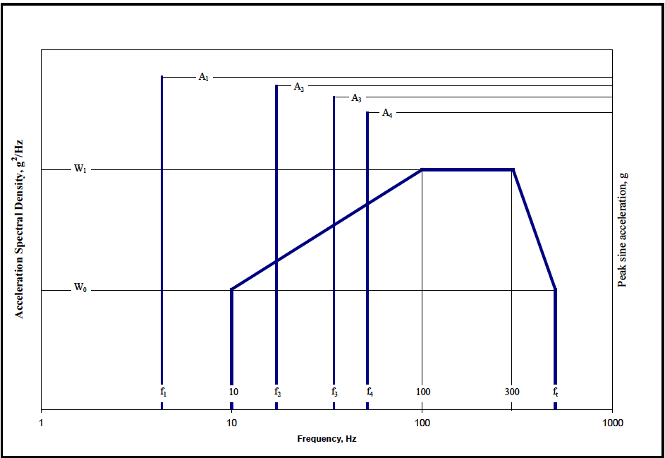
Figure description:
Vibration Specification Chart
Acceleration Spectral Density and Peak Sine Acceleration vs. Frequency
Legend
- Acceleration Spectral Density Envelope — color: blue; symbol: Solid thick line
- Peak Sine Acceleration — color: blue; symbol: Vertical bars
Annotations
- A1 (text_label - position: Peak sine acceleration level at frequency f1)
- A2 (text_label - position: Peak sine acceleration level at frequency f2)
- A3 (text_label - position: Peak sine acceleration level at frequency f3)
- A4 (text_label - position: Peak sine acceleration level at frequency f4)
- W0 (text_label - position: Left y-axis level W0)
- W1 (text_label - position: Left y-axis level W1)
| Frequency (Hz) | Acceleration Spectral Density (g^2/Hz) | Peak sine acceleration (g) |
|---|---|---|
| f1 | A1 | |
| 10 | W0 | |
| f2 | A2 | |
| f3 | A3 | |
| f4 | A4 | |
| 100 | W1 | |
| 300 | W1 | |
| ft | W0 |
Notes: This log-log chart specifies vibration testing parameters. The blue solid line represents the random vibration Acceleration Spectral Density (ASD envelope with points at (10, W0, (100, W1, (300, W1, and (ft, W0. The blue vertical bars represent sinusoidal vibration peaks at frequencies f1, f2, f3, and f4 with acceleration levels A1, A2, A3, and A4 respectively.)))))
Figure 514.8D-4 Category 14 – Helicopter vibration (Same as Annex C, Figure 514.8C-15).
| Helicopter | MAIN ROTOR | TAIL ROTOR | ||
|---|---|---|---|---|
| Rotation Speed 1P (Hz) | Number of Blades n | Rotation Speed 1T (Hz) | Number of Blades m | |
| AH-1 | 5.40 | 2 | 27.7 | 2 |
| AH-6J | 7.95 | 5 | 47.3 | 2 |
| AH-6M | 7.92 | 6 | 44.4 | 4 |
| AH-64 (early) | 4.82 | 4 | 23.4 | 4 |
| AH-64 (late) | 4.86 | 4 | 23.6 | 4 |
| CH-47D | Refer to TOP 01-2-603 (Paragraph 6.1, reference xx) | |||
| MH-6H | 7.80 | 5 | 47.5 | 2 |
| OH-6A | 8.10 | 4 | 51.8 | 2 |
| OH-58A/C | 5.90 | 2 | 43.8 | 2 |
| OH-58D | 6.60 | 4 | 39.7 | 2 |
| UH-1 | 5.40 | 2 | 27.7 | 2 |
| UH-60 | Refer to TOP 01-2-603 (Paragraph 6.1, reference xx) | |||
| MATERIEL | RANDOM LEVELS | SOURCE FREQUENCY (fx) RANGE (Hz) | PEAK ACCELERATION (Ax) at fx (GRAVITY UNITS (g)) | |
|---|---|---|---|---|
| General | W0 = 0.0010 g2/Hz W1 = 0.010 g2/Hz ft = 500 Hz | 3 to ≤ 10 | 0.70/(10.70 - fx) | |
| >10 to 25 | 0.10 x fx | |||
| 25 to 40 | 2.50 | |||
| 40 to 50 | 6.50 - 0.10 x fx | |||
| 50 to 500 | 1.50 | |||
| Instrument Panel | W0 = 0.0010 g2/Hz W1 = 0.010 g2/Hz ft = 500 Hz | 3 to ≤ 10 | 0.70/(10.70 - fx) | |
| >10 to 25 | 0.070 x fx | |||
| 25 to 40 | 1.750 | |||
| 40 to 50 | 4.550 - 0.070 x fx | |||
| 50 to 500 | 1.050 | |||
| External Stores | W0 = 0.0020 g2/Hz W1 = 0.020 g2/Hz ft = 500 Hz | 3 to ≤ 10 | 0.70/(10.70 - fx) | |
| >10 to 25 | 0.150 x fx | |||
| 25 to 40 | 3.750 | |||
| 40 to 50 | 9.750 - 0.150 x fx | |||
| 50 to 500 | 2.250 | |||
| On/Near Drive System Elements | W0 = 0.0020 g2/Hz W1 = 0.020 g2/Hz ft = 2000 Hz | 5 to ≤ 50 | 0.10 x fx | |
| > 50 to 2000 | 5.0 + 0.010 x fx | |||
| Main or Tail Rotor Frequencies (Hz) Determine 1P and 1T from the Specific Helicopter or from the table (below). | Drive Train Component Rotation Frequency (Hz) Determine 1S from Specific Helicopter and Component. | |||
| f1 = 1P | f1 = 1T | fundamental | f1 = 1S | fundamental |
| f2 = n x 1P | f2 = m x 1T | blade passage (BP) | f2 = 2 x 1S | 2nd harmonic |
| f3 = 2 x n x 1P | f3 = 2 x m x 1T | 2nd harmonic | f3 = 3 x 1S | 3rd harmonic |
| f4 = 3 x n x 1P | f4 = 3 x m x 1T | 3rd harmonic | f4 = 4 x 1S | 4th harmonic |
MIL-STD-810H METHOD 514.8, ANNEX D
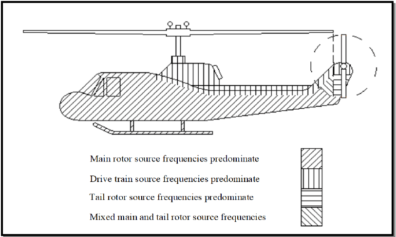
Figure description:
- Figure 514.8D-5: Category 14 - Helicopter vibration zones.
- Main rotor source frequencies predominate: Diagonally hatched area covering the main cockpit and fuselage.
- Drive train source frequencies predominate: Vertically hatched area located directly below the main rotor hub.
- Tail rotor source frequencies predominate: Horizontally hatched area located at the tail rotor assembly.
- Mixed main and tail rotor source frequencies: Cross-hatched area located on the tail boom transition and vertical stabilizer.
Figure 514.8D-5 - Category 14 - Helicopter vibration zones (Same as Annex C, Figure 514.8C-16).
514.8-2.3 Parametric Upper Limit Statistical Estimate Assumptions
In all the formulas for the estimate of the statistical upper limit of a set of N predictions or measurements,
it is assumed that (1) the estimates will be logarithm transformed to bring the overall set of measurements closer to those sampled of a normal distribution and (2) the measurement selection bias error is negligible. Since the normal and “t” distribution are symmetric, the formulas below apply for the lower bound by changing the sign between the mean and the standard deviation quantity to minus. It is assumed here that all estimates are at a single frequency or for a single bandwidth, and that estimates among bandwidths are independent so that each bandwidth under consideration may be processed individually, and the results summarized on one plot over the entire bandwidth as a function of frequency. For
y; = log10(x;)_i=1,2,∙∙∙ N
Mean estimate for true mean, μ, is given by
1 My N i=1
MIL-STD-810H
METHOD 514.8, ANNEX F, APPENDIX B
and the unbiased estimate of the standard deviation for the true standard deviation σ, is given by
514.8-2.3 Time Block Drop (Step 3)
Given fixed start and end times, data block size, and overlap percentage, the number and order of data blocks is also fixed. There is the possibility of corrupt data, or bad blocks, within the identified data segment (i.e., momentary telemetry dropouts, off speed sections, shock event, etc.). The analyst must be able to identify specific data blocks for exclusion in the subsequent spectral computations. To prevent discontinuities in the data, the blocks should not be deleted from the time data, but simply excluded during ASD calculation. In the event that the amount of measured data is limited, the analyst may be required to salvage available data through careful removal of limited dropouts in the data set that can be proven to be non-mechanical in nature (i.e., telemetry dropouts). Such manipulation is always a last resort and should be conducted by an experienced analyst.
Modern vibration control systems produce drive signals with Gaussian amplitude distributions. Therefore, the block drop utility should be implemented to warn the analyst if a particular block is grossly non-Gaussian in nature. One possible approach if to calculate the Crest Factor, Skewness, and Kurtosis of each block, and warn the analyst if user defined threshold values were exceeded. The analyst should then have the option to accept or reject that block. If a data set is highly non-stationary or non-Gaussian in nature a TWR test may be recommended in lieu of a classical spectral based vibration test.
The number of averages comprising a given ASD may vary as a function of the event time. For statistical relevance, a minimum of thirty-two (32) valid data blocks is recommended for ASD calculation. For any event consisting of less than 32 averages after block drop, 50 percent overlap can be used to effectively double the number of blocks available.
2.3.1 Climatic conditions
Many laboratory vibration tests are conducted under standard ambient test conditions as discussed in Part One, paragraph 5. However, when the life cycle events being simulated occur in environmental conditions significantly different than standard conditions, consider applying those environmental factors during vibration testing. Individual climatic test methods (Methods 501.6 and 502.6) of this Standard include guidance for determining levels of other
environmental loads. For temperature-conditioned environmental tests, (high temperature tests of explosive or energetic materials in particular), consider the materiel degradation due to extreme climatic exposure to ensure the total test program climatic exposure does not exceed the life of the materiel. (See Part One, paragraph 5.19.)
514.8-2.3.1 Random vibration
Random vibration is expressed as auto spectral density (also referred to as power spectral density, or PSD). The auto spectral density (ASD) at a given frequency is the square of the root mean square (rms) value of the acceleration, divided by the bandwidth of the measurement. Accuracy of spectral values depends on the product of the measurement bandwidth and the time over which the spectral value is computed. The normalized random error for a spectral estimate is given by 1/√BT, where B is the analysis bandwidth in Hz, and T is the averaging time in seconds. In general, use the smallest practical bandwidth or minimum frequency resolution bandwidth. Most commercially available vibration control systems assume that the acceleration amplitude has a normal (Gaussian) distribution. Other amplitude distributions may be appropriate in specific cases. Ensure that test and analysis hardware and software are appropriate when non-Gaussian distributions are encountered (refer to Method 525.1).
- a. Frequency range. ASD is defined over a relevant frequency range. This range is between the lowest and highest frequencies at which the materiel may be effectively excited by mechanical vibration. Typically, the low frequency is one half the frequency of the lowest resonance of the materiel, or the lowest frequency at which significant vibration exists in the environment. The high frequency is two times the highest materiel resonant frequency, the highest frequency at which significant vibration exists in the environment, or the highest frequency at which vibration can be effectively transmitted mechanically. Historically due to limitations in fixture transmissibility and shaker resonances, testing has been limited to a high frequency of 2000 Hz for mechanically transmitted vibration. However this limitation has changed with some facilities now performing system level tests to 3000 Hz and component level tests to 4000 Hz. When higher frequencies are needed, it may be necessary to augment the vibration with acoustic noise (see Method 523.4).
- b. Rms values. The use of rms values to specify random vibration is not sufficient. The spectrum rms value is the square root of the area under the spectral density curve over the total frequency range. It contains no frequency information. Rms values are useful as a general error check, and as a measure of power needed to run a vibration shaker. Definitions of vibration should always include frequency spectra.
514.8-2.3.1 NTL - Upper Normal One-Sided Tolerance Limit
The upper normal one-sided tolerance limit on the proportion of population values that will be exceeded with a confidence coefficient, , is given by , where
where is the one-sided normal tolerance factor given in Table 514.8F-B.I for selected values of , and . NTL is termed the upper one-sided normal tolerance interval (of the original set of estimates) for which percent of the values will lie below the limit with percent confidence. For and , this is referred to as the 95/50 limit.
The following table from reference g, contains the value for selected , and . In general this method of estimation should not be used for small with values of and close to 1 since it is likely the assumption of the normality of the logarithm transform of the estimates will be violated.
MIL-STD-810H
METHOD 514.8, ANNEX F, APPENDIX B
| N | γ = 0.50 | γ = 0.90 | γ = 0.95 | ||||||
|---|---|---|---|---|---|---|---|---|---|
| β = 0.90 | β = 0.95 | β = 0.99 | β = 0.90 | β = 0.95 | β = 0.99 | β = 0.90 | β = 0.95 | β = 0.99 | |
| 3 | 1.50 | 1.94 | 2.76 | 4.26 | 5.31 | 7.34 | 6.16 | 7.66 | 10.55 |
| 4 | 1.42 | 1.83 | 2.60 | 3.19 | 3.96 | 5.44 | 4.16 | 5.14 | 7.04 |
| 5 | 1.38 | 1.78 | 2.53 | 2.74 | 3.40 | 4.67 | 3.41 | 4.20 | 5.74 |
| 6 | 1.36 | 1.75 | 2.48 | 2.49 | 3.09 | 4.24 | 3.01 | 3.71 | 5.06 |
| 7 | 1.35 | 1.73 | 2.46 | 2.33 | 2.89 | 3.97 | 2.76 | 3.40 | 4.64 |
| 8 | 1.34 | 1.72 | 2.44 | 2.22 | 2.76 | 3.78 | 2.58 | 3.19 | 4.35 |
| 9 | 1.33 | 1.71 | 2.42 | 2.13 | 2.65 | 3.64 | 2.45 | 3.03 | 4.14 |
| 10 | 1.32 | 1.70 | 2.41 | 2.06 | 2.57 | 3.53 | 2.36 | 2.91 | 3.98 |
| 12 | 1.32 | 1.69 | 2.40 | 1.97 | 2.45 | 3.37 | 2.21 | 2.74 | 3.75 |
| 14 | 1.31 | 1.68 | 2.39 | 1.90 | 2.36 | 3.26 | 2.11 | 2.61 | 3.58 |
| 16 | 1.31 | 1.68 | 2.38 | 1.84 | 2.30 | 3.17 | 2.03 | 2.52 | 3.46 |
| 18 | 1.30 | 1.67 | 2.37 | 1.80 | 2.25 | 3.11 | 1.97 | 2.45 | 3.37 |
| 20 | 1.30 | 1.67 | 2.37 | 1.76 | 2.21 | 3.05 | 1.93 | 2.40 | 3.30 |
| 25 | 1.30 | 1.67 | 2.36 | 1.70 | 2.13 | 2.95 | 1.84 | 2.29 | 3.16 |
| 30 | 1.29 | 1.66 | 2.35 | 1.66 | 2.08 | 2.88 | 1.78 | 2.22 | 3.06 |
| 35 | 1.29 | 1.66 | 2.35 | 1.62 | 2.04 | 2.83 | 1.73 | 2.17 | 2.99 |
| 40 | 1.29 | 1.66 | 2.35 | 1.60 | 2.01 | 2.79 | 1.70 | 2.13 | 2.94 |
| 50 | 1.29 | 1.65 | 2.34 | 1.56 | 1.96 | 2.74 | 1.65 | 2.06 | 2.86 |
| ∞ | 1.28 | 1.64 | 2.33 | 1.28 | 1.64 | 2.33 | 1.28 | 1.64 | 2.33 |
2.3.2 Test item configuration
Configure the test item for each test as it will be in the corresponding life cycle phase. In cases representing transportation, include all packing, shoring, padding, or other configuration modifications of the particular shipment mode. The transportation configuration may be different for different modes of transportation.
- a. Loose cargo. The procedure contained herein is a general representation based on experience as well as measurement, and is not tailorable (see Annex C, paragraph 2.2 for details). The most realistic alternative for truck, trailer, or other ground transportation is to use Procedure II that requires the transportation vehicle and a full cargo load. In this test, the cargo has freedom to bounce, scuff and collide with other cargo and with the sides of the vehicle. The loose cargo environment includes conditions experienced by cargo transported in a vehicle traversing irregular surfaces. This test replicates the repetitive impact environment incurred by cargo transported under these conditions.
- b. Secured cargo. Procedure I assumes no relative motion between the vehicle cargo deck or cargo compartment and the cargo. This applies directly to materiel that is tied down or otherwise secured such that no relative motion is allowed considering vibration, shock, and acceleration loads. When restraints are not used or are such as to allow limited relative motions, provide allowance in the test setup and in the vibration excitation system to account for this motion. Procedure III is an alternative for ground transportation.
- c. Stacked cargo. Stacking or bundling of sets or groups of materiel items may affect the vibration transmitted to individual items. Ensure the test item configuration includes appropriate numbers and groupings of materiel items.
514.8-2.3.2 Sinusoidal vibration
Sine vibration is expressed as acceleration and a frequency. An environment dominated by sine vibration is characterized by a fundamental frequency and harmonics (multiples) of that fundamental. Often there will be more than one fundamental frequency. Each fundamental will generate harmonics. The service vibration environment in some cases (low performance propeller aircraft and helicopters for example) contains excitation that is basically sinusoidal in nature, and with a very low broadband background. The excitation derives from engine rotational speeds, propeller and turbine blade passage frequencies, rotor blade passage, and their harmonics. Environments such as this may be best simulated by a sinusoidal test. Ensure the frequency range of the sinusoidal exposure is representative of the platform environment. In many cases the broadband random may be of sufficient amplitude that the concept of simply omitting the broadband energy and conducting a pure sine test is either questionable or not acceptable. If so, refer to paragraph 2.3.3.
514.8-2.3.2 NPL - Upper Normal Prediction Limit
The upper normal prediction limit is the value of X (for the original data set) that will exceed the next predicted or measured value with confidence coefficient, 7, and is given by
My+o+N-1;a NPL (N,y)=10
where α=1-y and N-1;α is the student † distribution variable with N-1 degrees of freedom at the 100α=100(1-7) percentage point of the distribution. This estimate, because of the assumptions behind its derivation, requires careful interpretation relative to measurements made in a given location or over a given zone (reference g).
2.3.3 Multiple Exciter Consideration
Method 527.1 addresses scenarios in which the test item size requires use of more than one exciter or test fidelity requires more than one mechanical degree-of-freedom. In general, if a test facility has the capability to address more than one mechanical degree-of-freedom, and if such testing can be conducted in a time and cost effective manner, multiple axis testing should be considered as a test option. If the default curves provided within various categories of Method 514.8 are used as reference curves in a multiple-axis test, it should be recognized that Cross Spectral Density (CSD) terms will be undefined. Method 527 recommends that the coherence terms be near zero. Some reduction in levels (e.g., lower conservatism factors) may be justified if it can be shown that the multiple degree-of-freedom (MDOF) test produces significantly higher stress levels or lower fatigue life than the sequential single degree-of-freedom (SDOF) tests.
514.8-2.3.3 Mixed broadband and narrowband vibration
In some cases, the vibration environment is characterized by quasi-periodic excitation from reciprocating or rotating structures and mechanisms (e.g., rotor blades, propellers, pistons). When this form of excitation predominates, source dwell vibration is appropriate. Source dwell is characterized by broadband random vibration, with higher level narrowband random, or sinusoidal vibration superimposed. Since data reduction techniques affect the apparent amplitudes of these different types of signals, exercise care when determining levels of random and sinusoidal vibration from measured data.
- a. Narrowband random over broadband random. Ensure that the amplitudes and frequencies of the total spectrum envelope the environment. The narrowband bandwidth(s) should encompass or be cycled through frequencies representative of variations of the environment and variations of materiel resonant frequency (see paragraph 2.4.3 below).
- b. Sinusoid(s) over broadband random background. Ensure the random spectrum is continuous over the frequency range, and that it envelopes all of the environment except for the amplitude(s) to be represented by the sinusoid(s). The sinusoid(s) amplitude(s) should envelope the sinusoid(s) in the environment. Cycle
MIL-STD-810H METHOD
2.3.4 Transient vibration
Transient vibration is a time-varying "windowed" portion of a random vibration that is of comparatively short duration (e.g., 0.5 second to 7.5 seconds). Currently, such a measured environment is replicated in the laboratory on a vibration exciter under waveform control. Verification of the laboratory test is provided by (1) display of the laboratory measured amplitude time history; (2) an optimally smooth estimate of the amplitude time history time-varying root- mean-square, and (3) either an energy spectral density estimate, or a Shock Response Spectrum (SRS) estimate for comparatively short environments (transient vibration duration less than the period of the first natural mode of the test item), or a time-varying auto spectral density estimate of longer duration environments, e.g., 2.5 to 7.5 seconds. In general, since the environment is being replicated in the laboratory under waveform control, if the impulse response function of the system is correctly determined and correctly applied, the replication should be nearly identical to the measured environment. The transient vibration environment is an important environment for stores resident in platform weapon bays that may be exposed to such environments many times in the life of training missions. See paragraph 6.1, references c and bb; Method 516.8; and Method 525.2 for procedures relative to transient vibration.
2.3.5 Random versus sinusoidal vibration equivalence
In the past, most vibration was characterized in terms of sinusoids. Currently, most vibration is correctly understood to be random in nature and is characterized as such. This results in a demand to determine equivalence between random and sine vibration. This demand is generated by the need to use materiel that was developed to sine requirements.
- a. General equivalence. Sine and random characterizations of vibration are based on distinctly different sets of mathematics. In order to compare the effects of given random and sine vibration on materiel, it is necessary to know the details of materiel dynamic response. A general definition of equivalence is not feasible.
- b. G-rms. Often, attempts are made to compare the peak acceleration of sine to the rms acceleration of random. The only similarity between these measures is the dimensional units that are typically acceleration in standard gravity units (g). Peak sine acceleration is the maximum acceleration at one frequency (see paragraph 2.3.2). Random rms is the square root of the area under a spectral density curve (see paragraph 2.3.1). These are not equivalent.
2.3.6 Combination of test spectra
When combining test spectra to develop an envelope or weighted average of multiple vibration profiles, refer to the discussion and techniques presented in Annex F of this method.
2.4 Test Item Operation
Where vibration tests are conducted to determine operational capability while exposed to the environment, operate the test item during the vibration test. Otherwise, verify operation before and after the vibration test. Use caution when applying combined or enveloped vibration profiles during operational tests as the levels may not be representative of any particular operational environment. During operational vibration tests, monitor and record sufficient data to define the achieved performance and sensitivity of the materiel to the vibration environment. See Annex A, paragraph 2.1.2.1 for additional functional test considerations.
514.8-2.4 Platform/Materiel and Fixture/Test Item Interaction
Generally, it is assumed that the vibration environment of the materiel is not affected by the materiel itself. That is, the vibration of the platform at the materiel attachment point would be the same whether or not the materiel is attached. Since the entire platform, including all materiel, vibrates as a system, this is not strictly correct. However, when the materiel does not add significantly to the mass or stiffness of the platform, the assumption is correct within reasonable accuracy. The following paragraphs discuss the limitations of this assumption. These effects also apply to sub- elements within materiel and to the interactions of materiel with vibration excitation devices (shakers, slip tables, fixtures, etc.).
514.8-2.4 Category 7 - Aircraft - jet
Cargo vibration environments on jet aircraft are broadband random in nature. The maximum vibrations are usually engine exhaust noise generated and occur during takeoff. Levels drop off rapidly after takeoff to lower level cruise levels that are boundary layer noise generated. These sources are discussed in Annex D, paragraph 2.1.
- a. Low frequency vibration. Vibration criteria typically begin at 15 Hz. At frequencies below 15 Hz, it is assumed that the cargo does not respond dynamically (see Annex A, paragraph 2.4). Airframe low frequency vibration (gust response, landing impact, maneuvers, etc.) is experienced as steady inertial loads (acceleration). That part of the environment is included in Method 513.8.
- b. Large cargo items. Cargo items that are large relative to the airframe in dimensions and/or mass may interact with aircraft structural dynamics (see Annex A, paragraph 2.4). This is particularly true if the materiel has natural frequencies below 20 Hz. This interaction may have serious consequences with regard to aircraft loads and flutter. Evaluate materiel that fits this description by the aircraft structural engineers prior to carriage. Contact the Aircraft Product Center Wings responsible for the aircraft type for this evaluation.
- c. Exposure levels.
- (1) Vibration qualification criteria for most jet cargo airplanes are available through the Aircraft Product Center Wings responsible for the aircraft type. These criteria are intended to qualify materiel for permanent installation on the airplanes and are conservative for cargo. However, function criteria for materiel located in the cargo deck zones can be used for cargo if necessary. The guidance of Annex D, paragraph 2.1 can also be used to generate conservative criteria for specific airplanes and cargo. The associated spectral shape and functional guidance from Annex D are repeated below for convenience as Figure 514.8C-10 and Table 514.8C-X.
- (2) Figure 514.8C-9 shows the cargo compartment zone functional qualification levels of the C-5, C/KC- 135, C-17, E/KE-3, KC-10, and T-43A aircraft. These are recommended criteria for jet aircraft cargo. Also, shown on the figure is a curve labeled "General Exposure." This curve is based on the worst case zone requirements of the most common military jet transports, so that even though it does not envelope all peaks in the various spectra, it should still be mildly conservative for cargo. Also, since it does not allow the valleys in the individual spectra, it should cover other jet transports with different frequency characteristics. The envelope represents take-off, the worst case for cargo. Vibration during other flight conditions is substantially less.
- d. Exposure durations. When Figure 514.8C-9 is used, select a duration of one minute per takeoff. Determine the number of takeoffs from the LCEP.
MIL-STD-810H METHOD 514.8, ANNEX C
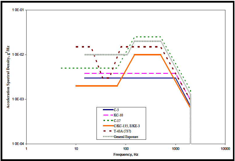
Figure description:
Acceleration Spectral Density vs Frequency
Legend
- C-5 — color: dark blue; symbol: Solid line
- KC-10 — color: magenta; symbol: Dashed line
- C-17 — color: dark green; symbol: Dotted line
- C/KC-135, E/KE-3 — color: orange; symbol: Solid line
- T-43A (737 — color: dark red; symbol: Dashed line
- General Exposure — color: grey; symbol: Dotted pattern line
| Frequency (Hz) | C-5 | KC-10 | C-17 | C/KC-135, E/KE-3 | T-43A (737) | General Exposure |
|---|---|---|---|---|---|---|
| 5 | null | null | 5.0E-03 | null | null | null |
| 10 | null | null | 5.0E-03 | 2.0E-03 | 1.5E-02 | null |
| 15 | 3.0E-03 | 4.0E-03 | 5.0E-03 | 2.0E-03 | 1.5E-02 | 1.0E-02 |
| 20 | 3.0E-03 | 4.0E-03 | 5.0E-03 | 2.0E-03 | 1.5E-02 | 1.0E-02 |
| 40 | 3.0E-03 | 4.0E-03 | 5.0E-03 | 2.0E-03 | 3.0E-03 | 1.0E-02 |
| 60 | 3.0E-03 | 4.0E-03 | 5.0E-03 | 2.0E-03 | 3.0E-03 | 1.0E-02 |
| 70 | 3.0E-03 | 4.0E-03 | 5.0E-03 | 2.0E-03 | 6.0E-03 | 1.0E-02 |
| 100 | 3.0E-03 | 4.0E-03 | 1.1E-02 | 4.5E-03 | 1.5E-02 | 1.0E-02 |
| 150 | 3.0E-03 | 4.0E-03 | 2.5E-02 | 1.0E-02 | 1.5E-02 | 2.0E-02 |
| 500 | 3.0E-03 | 4.0E-03 | 2.5E-02 | 1.0E-02 | 1.5E-02 | 2.0E-02 |
| 900 | 3.0E-03 | 4.0E-03 | 1.1E-02 | 3.5E-03 | 7.0E-03 | 8.0E-03 |
| 1000 | 2.5E-03 | 4.0E-03 | 9.0E-03 | 3.0E-03 | 5.0E-03 | 6.0E-03 |
| 2000 | 7.0E-04 | 1.0E-03 | 1.5E-03 | 6.0E-04 | 1.0E-03 | 1.2E-03 |
Notes: The chart is a log-log plot. All data series terminate abruptly at a frequency of 2000 Hz, as indicated by the vertical grey dotted line.
Figure 514.8C-9. Category 7 - Jet aircraft cargo vibration exposure.
| C-5 | KC-10 | KC-135, E-3 | C-17 | ||||||||
|---|---|---|---|---|---|---|---|---|---|---|---|
| Hz | g²/Hz | dB/Oct | Hz | g²/Hz | dB/Oct | Hz | g²/Hz | dB/Oct | Hz | g²/Hz | dB/Oct |
| 15 | 0.003 | 15 | 0.0038 | 10 | 0.002 | 5 | 0.005 | ||||
| 1000 | 0.003 | -6 | 1000 | 0.0038 | -6 | 67 | 0.002 | 6 | 67 | 0.005 | 6 |
| 2000 | 7.5E-4 | 2000 | 9.5E-4 | 150 | 0.01 | 150 | 0.025 | ||||
| rms = 2.11 g | rms = 2.38 g | 500 | 0.01 | -6 | 500 | 0.025 | -6 | ||||
| 2000 | 6.3E-4 | 2000 | 1.6E-3 | ||||||||
| rms = 2.80 g | rms = 4.43 g | ||||||||||
| T-43A (737) | General Exposure | Note: C-17 levels apply to the primary cargo floor. Levels for items carried on the aft ramp are higher. | |||||||||
| Hz | g²/Hz | dB/Oct | Hz | g²/Hz | dB/Oct | ||||||
| 10 | 0.015 | 15 | 0.01 | ||||||||
| 20 | 0.015 | -9 | 106 | 0.01 | 6 | ||||||
| 34 | 0.003 | 150 | 0.02 | ||||||||
| 47 | 0.003 | 9 | 500 | 0.02 | -6 | ||||||
| 80 | 0.015 | 2000 | 1.3E-3 | ||||||||
| 500 | 0.015 | -6 | rms = 4.02 g | ||||||||
| 2000 | 9.5E-4 | ||||||||||
| rms = 3.54 g | |||||||||||
MIL-STD-810H METHOD 514.8, ANNEX C
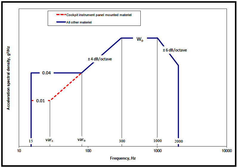
Figure description:
Legend
- Cockpit instrument panel mounted materiel — color: red; symbol: dashed line with dots
- All other materiel — color: blue; symbol: solid line
Annotations
- 0.04 (text_label - position: y = 0.04)
- 0.01 (text_label - position: y = 0.01)
- ± 4 dB/octave (text_label - position: slope between var_o and 300 Hz)
- W_o (text_label - position: y = W_o, between 300 and 1000 Hz)
- ± 6 dB/octave (text_label - position: slope between 1000 and 2000 Hz)
- 15 (vertical_line - position: x = 15)
- var_c (vertical_line - position: x = var_c)
- var_o (vertical_line - position: x = var_o)
- 300 (vertical_line - position: x = 300)
- 1000 (vertical_line - position: x = 1000)
- 2000 (vertical_line - position: x = 2000)
| Frequency, Hz | All other materiel () | Cockpit instrument panel mounted materiel () |
|---|---|---|
| 15 | 0.04 | null |
| varc | 0.04 | 0.01 |
| varo | 0.04 | 0.04 |
| 300 | Wo | Wo |
| 1000 | Wo | Wo |
| 2000 | (slope: -6 dB/octave) | (slope: -6 dB/octave) |
Notes: The graph shows acceleration spectral density (g²/Hz versus frequency (Hz for two categories of material. Key points on the frequency axis are 15, var_c, var_o, 300, 1000, and 2000. Key values on the spectral density axis are 0.01, 0.04, and W_o. Slopes are defined in dB/octave.))
Figure 514.8C-10. Category 7 - Jet aircraft vibration exposure. (Same as Annex D, Figure 514.8D-1.)
| W0 = WA + Σ1n(WJ) | |
|---|---|
| W0, WA, WJ - Exposure levels in acceleration spectral density (g²/Hz). | |
| Aerodynamically induced vibration | |
| WA = a × b × c × (q)² | |
| Jet engine noise induced vibration | |
| WJ = {[0.48 × a × d × cos²(θ)/R] × [Dc × (Vc / Vr)³ + Df × (Vf / Vr)³]} | |
| a - Platform / Materiel interaction factor (see Annex A, paragraph 2.4). Note that this factor applies to W0 and not to the low frequency portion (15 Hz to break) of Figure 514.8C-10. | |
| = 1. 0 for materiel mounted on vibration isolators (shock mounts) and materiel weighing less than 36.3 kg. | |
| = 1.0 ×10(0.6 - W / 60) for materiel weighing between 36.3 and 72.6 kg.(w = weight in kg) | |
| = 0. 25 for materiel weighing 72.6 kg or more. | |
| b - Proportionality factor between vibration level and dynamic pressure (SI units). | Σ1n - Jet noise contribution is the sum of the WJ values for each engine. |
| = 2.96 ×10⁻⁶ for materiel mounted on cockpit instrument panels. | d - Afterburner factor. = 1. 0 for conditions where afterburner is not used or is not present. = 4. 0 for conditions where afterburner is used. |
| = 1.17 ×10⁻⁵ for cockpit materiel and materiel in compartments adjacent to external surfaces that are smooth and free from discontinuities. | R - Vector distance from center of engine exhaust plane to materiel center of gravity, m (ft). |
| = 6.11 ×10⁻⁵ for materiel in compartments adjacent to or immediately aft of external surface discontinuities (cavities, chines, blade antennae, speed brakes, etc.), fuselage aft of wing trailing edge, wing, empennage, and pylons. | θ - Angle between R vector and engine exhaust vector (aft along engine exhaust centerline), degrees For 70°< θ ≤ 180° use 70°. |
| c = Mach number correction. Note that this factor applies to W0 and not to the low frequency portion (15 Hz to varc or varo) of Figure 514.8C-10. | Dc - Engine core exhaust diameter, m (ft). |
| = 1. 0 for 0 ≤ Mach ≤ 0. 9 | Df - Engine fan exhaust diameter, m (ft). |
| = (-4.8M + 5.32) for 0.9 ≤ Mach ≤1. 0 (where M = Mach number) | Vr - Reference exhaust velocity, m/sec (ft/sec). = 564 m/sec |
| = 0.52 for Mach number greater than 1.0 | Vc - Engine core exhaust velocity (without afterburner), m/sec (ft/sec). |
| q - Flight dynamic pressure, kN / m² (lb/ft²). | Vf - Engine fan exhaust velocity (without afterburner), m/sec (ft/sec). |
| varc - intersection frequency for cockpit materiel based on 4dB/oct slope from W0 | |
| varo - intersection frequency for all other materiel based on 4dB/oct slope from W0 | |
| (See Annex A, para. 2.6.1 and Table 514.8D-V) | |
| If Dimensions are in feet and pounds then: | |
| a = 1. 0 for materiel mounted on vibration isolators (shock mounts) and materiel weighing less than 80 lb. | |
| = 1.0 ×10(0.60 - 0.0075 W) for materiel weighing between 80 and 160 lb. | |
| = 0. 25 for materiel weighing 160 lb. or more. | |
| b = 6.78 ×10⁻⁹, 2.70 ×10⁻⁸, or 1.40 ×10⁻⁷ in the order listed above. | |
| Vr = 1850 feet/second | |
514.8-2.4 Category 15 - Aircraft stores - assembled, jet aircraft
Assembled jet aircraft stores may encounter three distinct vibration environments; external captive carriage, internal captive carriage, and free flight.
Note: High frequency vibration (above 1000 Hz) cannot be practically transmitted to a store mechanically. Combine store vibration and acoustic testing (Method 523.4). These test excitations in combination produce a much more realistic test.
514.8-2.4 Nonparametric Upper Limit Statistical Estimate Assumptions
If there is some reason to believe that the data, after it has been logarithm-transformed, will not be sufficiently normally distributed to apply the parametric limits defined above, consideration must be given to nonparametric limits, i.e., limits that are not dependent upon assumptions concerning the distribution of estimate values. In this case there is no need to transform the data estimates. All of the assumptions concerning the selection of estimates are applicable for nonparametric estimates. With additional manipulation, lower bound limits may be computed.
514.8-2.4 Calculate ASD Average (Step 4)
Once the data blocks for processing are selected, a single-event ASD sum-set is generated for each channel and each event. A single-event ASD sum-set includes five ASDs, an average, peak hold, standard deviation, sum, and spectral spike removed, as defined in Table 514.8F-D.II. The first four ASDs of the sum-sets are calculated during Step 4. The average, denoted as ASD(Avg), is a standard n average ASD, where n is the number of data blocks selected for processing during block drop. Individual ASDs are calculated for each data block and then averaged on a spectral line basis to produce the ASD(Avg). The ASD(Sum) is calculated by adding Nₑ standard deviations to the ASD(Avg), where Nₑ is a user selected value typically set to 1. The ASD(Sum) becomes the working ASD and is passed forward to the next step. Use of the ASD(Sum) is intended to address severity variance across the vehicle fleet of interest. To minimize overly high ASD(Sum) levels, due for example to high standard deviations resulting from ground vehicle speed fluctuations, the ASD(Sum) is constrained to be no higher than Mₑ *ASD(Avg) where Mₑ is a user defined parameter typically set to 2. The ASD(Sum) is also limited to the ASD(Peak) level at each spectral line. In the rare scenario in which there exists specific information as to how the vehicle being used to acquire the test data compares to the fleet, the Parameter Nₑ should be customized accordingly.
MIL-STD-810H MIL STD 883A
METHOD 514.8, ANNEX F, APPENDIX D
| Nomenclature | Definition |
|---|---|
| ASD(Avg) | A standard nd average ASD. (See Gm (f) as defined in Appendix B) |
| ASD(Peak) | Calculated by holding the maximum amplitude of each spectral line over nd averages. (See Gp (f) as defined in Appendix B) |
| ASD(Stdv) | Calculated by determining the standard deviation of each spectral line over n averages. (See Gd (f) as defined in Appendix B) |
| ASD(Sum) | Calculated by adding Ne standard deviations to the average for each spectral line. ASD(Sum) = Ne *ASD(Stdv) + ASD(Avg) Ne is a user defined variable typically set to 1. ASD(Sum) is limited by ASD(Peak) and Me *ASD(Avg) where Me is a user defined variable typically set to 2. (See Gs (f) as defined in Appendix B) |
| ASD(SpkRmvd) | ASD(Sum) after Frequency Spectral spike Removal. |
2.4.1 Mechanical impedance
- a. Large mass items. At platform natural frequencies where structural response of the platform is high, the materiel will load the supporting structures. That is, the mass of the materiel is added to the mass of the structure, and it inertially resists structural motions. If the materiel mass is large compared to the platform mass, it causes the entire system to vibrate differently by lowering natural frequencies and changing mode shapes. If the materiel inertia is large compared to the stiffness of the local support structure, it causes the local support to flex, introducing new low frequency local resonances. These new local resonances may act as vibration isolators (see paragraph 2.4.2 below).
MIL-STD-810H METHOD
514.8-2.4.1 Captive flight - external carriage
Vibration (for gunfire induced vibration, see Method 519.7) experienced by a store carried externally on a jet aircraft arises primarily from four sources:
-
a. Engine noise is produced by turbulence in the boundary of the jet exhaust plume. This turbulence is maximum at initiation of takeoff when the velocity difference between the jet and ambient air is maximum. This source is generally of primary importance when the store is carried on an aircraft that uses pure jet or very low bypass engines since these engines have the highest exhaust velocities. Further, it is important at higher frequencies because sources discussed below dominate at lower frequencies (paragraph 6.1, references u, v, and w).
-
b. In-flight store vibration is primarily caused by aerodynamic turbulence distributed over the surface of the store.
-
(1) In single carriage, excitation is relatively independent of the carrying aircraft and mounting location on the aircraft. Local flow disturbances such as pylon wakes will vary considerably between aircraft and between store stations on a given aircraft. In general, these do not greatly affect overall store vibration. However, they may severely affect local structures such as tail fins that, in turn, may increase levels of store vibration. See Annex E, paragraph 2.1.2 for guidance on local flow effects. When stores are carried close together, the turbulence field around each is increased. A store carried behind another store is exposed to the turbulence generated by the forward store.
-
(2) An extensive program of measurement and analysis was accomplished to characterize this environment (paragraph 6.1, references u, v, and w). Vibratory excitation is influenced by store configuration, structural configuration, mass density, and flight dynamic pressure. The high frequency portion of the resulting vibration is best represented by a combination of mechanical vibration and the acoustic noise exposures of Method 523.4. The low and medium frequency portion of this environment is better simulated by mechanical excitation. The studies mentioned above resulted in a method to accomplish this defining the response vibration of the store rather than specifying input vibration. This Method also includes low frequency vibration transmitted from the carrying aircraft (see below).
-
c. Vibrations of the carrying aircraft are transmitted to the store through the attaching structures. The total vibrating system (aircraft, pylon, bomb rack, and store) is a low frequency system. That is, the lowest natural frequency of the system is typically below 20 Hertz and the store is isolated from high frequency aircraft vibration. Depending on the particular circumstances, these vibrations are often best represented as transient vibration (see Annex A, paragraph 2.3.4).
-
(1) The low frequency vibration of the airframe transmitted to the store is not separable in the general case from the low frequency turbulence generated vibration. This vibration is accounted for by the method discussed under “Aerodynamic turbulence” (paragraph 2.4.1b).
-
(2) Flight test measurements on the F-15 with various external stores, (paragraph 6.1, reference x) have shown intense, very low frequency vibrations associated with aircraft buffet during high angle of attack maneuvers. Other aircraft, such as F-14, F-16, and F-18, or next generation fighters, have the potential to produce intense buffet vibrations during maneuvers.
-
(3) The F-15 buffet maneuver envelope is roughly bounded by speeds of 0.7 to 1.0 Mach and altitudes of approximately 3 to 10.7 kilometers (10,000 to 35,000 ft). Flight test measurements have shown the maximum F-15 buffet vibration to occur in the flight regime of 0.8 to 0.9 Mach, 4.6 to 7.6 km (15,000 to 25,000 ft) altitude, 8° to 12° angle of attack, and dynamic pressure less than 26.3 kN/m2 (550 lb/ft2). Similar measurements on F/A-18 have shown the maximum buffet maneuver vibration to occur in the regime of 0.85 to 0.95 Mach, 1.5 to 4.6 km (5,000 to 15,000 ft.), 8° to 10° angle of attack, and dynamic pressure less than 33.5 kN/m2 (700 lb/ft2). Although the vibration levels during high-performance maneuvers are very intense, they generally do not last for more than 10 seconds, reaching maximum in less than a second and deteriorating in 5 to 10 seconds. Typically, F-15 external stores will experience 30 seconds of maneuver buffet vibration for each hour of captive-carriage flight.
-
(4) Buffet vibration is typically concentrated between 10 and 50 Hz. Vibration response of the store is dominated by store structural resonances. Store loads that occur at frequencies below the lowest store natural frequency are effectively static loads. Buffet levels vary over a wide range on a given aircraft as well as between aircraft. Thus, buffet vibration requirements should be derived from in-flight vibration measurement when possible. As an alternative to measurements, the lowest store vibratory modes can be exercised at conservative levels to show that the store will be robust enough for any encountered buffet vibration. This does not cover the static loads associated with buffet. In order to include these loads, it is necessary to duplicate flight measured dynamic bending moments as discussed as an option in the front part of this Method (paragraph 4.2.1.2, Force control strategy). This would require extending the test frequency down to the lowest frequency of airplane buffet response and must be done in coordination with the responsible strength and loads engineers.
-
d. Stores are also susceptible to vibration generated by internal materiel and local aerodynamic effects. There are no accepted criteria or methodology for predicting these environments. However, these environments can be dominating vibration sources and should not be ignored. Whenever they are present, they should be accounted for through development tests and measurements.
-
(1) Internal materiel vibration is typically produced by rotating elements such as electric or hydraulic motors. Any device that generates or incorporates physical motion can produce vibration. Ram air turbines (RAT) are sometimes used to generate electrical or hydraulic power. A RAT can produce high levels of rotating element vibration in addition to severe aerodynamic turbulence at and behind the rotating blades.
-
(2) Acoustic resonance of simple cavities is typically handled as an acoustic environment (see Method
515.8). Any hole, cavity, opening, inlet, etc., that allows airflow to enter the store or a cavity in the store can produce high intensity acoustic resonance responses.
514.8-2.4.1 ENV - Upper Limit
The maximum upper limit is determined by selecting the maximum estimate value in the data set.
MIL-STD-810H
METHOD 514.8, ANNEX F, APPENDIX B
The main disadvantage of this estimate is that the distributional properties of the estimate set are neglected so that no probability of exceedance of this value is specified. In the case of outliers in the estimate set, may be far too conservative. is also sensitive to the bandwidth of the estimates.
2.4.2 Vibration isolation
Vibration isolators (shock mounts), isolated shelve, and other vibration isolation devices add low-frequency resonances to the dynamic system that attenuate high-frequency vibration inputs to materiel. Vibration inputs at the isolation frequencies (materiel six degree-of-freedom rigid body modes) are amplified, resulting in substantial rigid body motions of the isolated materiel. Effective performance of these devices depends on adequate frequency separation (minimum factor of two) between materiel resonant frequencies and isolation frequencies, and on adequate sway space (clearance around isolated materiel) to avoid impacts of the isolated materiel with surrounding materiel (possibly also vibration isolated and moving) and structure.
- a. Sway space. Include sway amplitude and isolation characteristics (transmissibility versus frequency) in all design analyses and measure them in all vibration tests. Isolation devices are nonlinear with amplitude. Evaluate these parameters at vibration levels ranging from minimum to maximum. These comments also apply to isolated sub-elements within materiel items.
- b. Minimum ruggedness. All materiel should have a minimum level of ruggedness, even if protected by isolation in service use and shipping. Thus, when materiel development does not include all shipping and handling environments of the materiel’s life cycle, include the appropriate minimum integrity exposures in materiel (Annex E, paragraph 2.1.1).
514.8-2.4.2 Captive flight – internal carriage
There are two distinct vibration environments for stores carried in a closed, internal, aircraft bay. These environments occur when the bay is closed to the aircraft external environment and when the bay is open to this environment. Aircraft capable of high angle of attack maneuvers may be susceptible to buffet. Since buffet vibration is mechanically transmitted to the store, the bay will provide no protection. Thus the buffet vibration method discussed above applies.
- a. The general vibration environment of a store in a closed bay is very mild. The store is protected from the jet engine noise and aerodynamic turbulence environments and isolated from aircraft vibration. If a store is qualified for external carriage on any jet aircraft, this should more than adequately account for this case. There is no known method to predict this environment for the general case. Measured data may be available for specific aircraft, but generally measurements will be necessary if this environment must be defined.
- b. When the bay is opened in flight, a dramatic event occurs. This event is referred to as cavity resonance (paragraph 6.1, references l and m) and results in high levels of turbulence inside the bay. This is wide band turbulence with very high spikes across the spectrum, unless suppression devices are installed in the bay. The low frequency portions of the disturbance are not likely to drive the store because disturbance wavelengths greatly differ from store dimensions. The high frequency part of the spectrum will significantly affect the store. Store vibration resulting from this turbulence cannot be adequately predicted. Acoustic characterizations of the turbulence exist for most active aircraft and the resulting vibration is best represented by the acoustic noise exposures of Method 515.8.
- (1) Generally, store flight surfaces (control surfaces, wings, stabilizers, etc.) are small enough (small surface area) and/or stiff enough (lowest resonant frequency above 100 Hz) that they are not significantly excited by this environment. However, in cases in which the control surfaces of the store are relatively large or soft, they may be excited by the open-bay environment. In these cases the store response can result in flight surface failure, high levels of store vibration, or both.
- (2) In some instances, a store is carried in one configuration or position until use. Just prior to use, the configuration or position may change. For example, a weapon carried on a rotary launcher inside a weapons bay of a large bomber. The weapon moves from clock position to clock position as other weapons on the launcher are launched. The weapon is exposed to the open bay environment either each time another weapon is launched, or for a relatively long period while several are launched. Another example is a weapon that is extended out of the bay on the launch mechanism prior to launch. Here the environment will change considerably with position. A third example is an optical sensor pod. This type of store can be carried internally, extended into the air stream, configuration changed (e.g., covers over optical windows retract), operated, configuration changed back, and retracted into the closed bay many times in a lifetime. Account for such variations in environment and configuration.
Note: Door opening, position changes, configuration changes, door closing, etc., should be expected to happen rapidly. Each of these events and, possibly, a whole sequence of events can happen rapidly enough, so that they should be treated as transient (see Annex A, paragraph 2.3.4, and Method 516.8) rather than steady state vibration.
2.4.3 Materiel resonant frequency variation
The installed resonant frequencies of materiel may vary from those of the laboratory test. One cause is the small variations between serial items from an assembly process. Tightness of joints, slight differences in dimensions of parts and subassemblies, and similar differences affect both the resonant frequencies and the damping of the various modes of the item. A second cause is the interaction between the materiel and the mounting. As installed for field use, a materiel item is tied to mounting points that have an undefined local flexibility, and that move relative to each other in six degrees of freedom as the platform structure vibrates in its modes. In a typical laboratory test, the test item is tied to a massive, very stiff fixture intended to transmit single axis vibration uniformly to each mounting point. In each case, the mounting participates in the vibration modes of the materiel item and, in each case, the influence is different. When defining test criteria, consider these influences. Both in the cases of measured data and arbitrary criteria, add an allowance to narrow band spectral elements.
514.8-2.4.3 Free flight
Vibration will be experienced by stores that are deployed from aircraft, ground vehicles, or surface ships. The sources of vibration for the free flight environment are engine exhaust noise, vibration, and noise produced by internal equipment and boundary layer turbulence.
- a. Generally, engine exhaust noise levels will be too low to excite significant vibration in the store. This is because the engine only operates when the ratio of the exhaust velocity to the ambient air speed is low and (except in unusual cases) the exhaust plume is behind the store.
- b. Vibration produced by onboard materiel can be severe in specific cases. Examples are ram air turbines, engines, and propellers. There is no general basis for predicting store vibrations from such sources. Each
case must be evaluated individually, and it is likely that measurements will be required.
- c. Boundary layer turbulence induced vibration should be as for captive carriage except that store vibration mode frequencies may shift, flight dynamic pressures may be different, and turbulence from the carrier aircraft and nearby stores will be absent.
2.4.4 Exposure levels
Select test levels and spectra for captive flight and free flight from Table 514.8D-IV and Figures 514.8D-6 and 514.8D-7. Buffet test spectra and levels are provided in Figure 514.8D-7. The use of these tables and figures is suggested only when there is an absence of satisfactory flight measurements. Except for buffet portions, these criteria are closely based in paragraph 6.1, references u, v, and w. These document the results of an extensive study and include a large amount of information and insight. The buffet criteria are based on paragraph 6.1, reference x, and additional measurements and experience with the F-15 aircraft. It represents F-15 wing pylon buffet that is the worst known buffet environment. F-15 fuselage store stations buffet environments are generally less severe. Criteria for the other environments must be determined for each specific case.
2.5 Modal Test and Analysis
Modal test and analysis is a technique for determining the structural dynamic characteristics of materiel and test fixtures. Modal tests (paragraph 6.1, reference cc), also known as ground vibration tests (GVT) and ground vibration surveys (GVS), apply a known dynamic input to the test item, and the resulting responses are measured and stored. Modal analysis methods are applied to the measured data to extract modal parameters (resonant frequencies, mode
MIL-STD-810H METHOD
514.8-2.5 Category 8 - Aircraft - propeller
Cargo vibration environments on propeller aircraft are dominated by relatively high amplitude, approximately sinusoidal spikes at propeller passage frequency and harmonics. There is wide band vibration at lower levels across the spectra. This wide band vibration is primarily due to boundary layer flow over the aircraft. These sources are discussed in Annex D, paragraph 2.2.
- a. Low frequency vibration. Vibration criteria typically begin at 10 Hz. At frequencies below 10 Hz it is assumed that the cargo does not respond dynamically (see Annex A, paragraph 2.4). Airframe low frequency vibration (gust response, landing impact, maneuvers, etc.) are experienced as steady inertial loads (acceleration). That part of the environment is included in Method 513.8.
- b. Large cargo items. Cargo items that are large relative to the airframe in dimensions and/or mass may interact with aircraft structural dynamics (see Annex A, paragraph 2.4). This is particularly true if the materiel has natural frequencies below 20 Hz. This interaction may have serious consequences with regard to aircraft loads and flutter. Materiel that fits this description must be evaluated by aircraft structural engineers prior to carriage. Contact the Aircraft Product Center Wing responsible for the aircraft type for this evaluation.
- c. Exposure levels. Whenever possible, use flight vibration measurements to develop vibration criteria. In the absence of flight measurements: use the spectra of Figure 514.8C-11 and Table 514.8C-XI for the 4-blade C-130; use the spectra of Figure 514.8C-12 and Table 514.8C-XII for the 6-blade C-130; and use the spectra of Figure 514.8C-13 and Table 514.8C-XIII for fixed wing propeller aircraft other than C-130. Zones for propeller aircraft are shown in Figure 514.8C8-14. The C-130 spectra are based on measurements made on several versions of the C-130K (4 blade) and C-130J (6-blade) aircraft (paragraph 6.1, references yy and zz) and are fairly representative of the environments of these aircraft.
- d. Exposure durations. Take durations from the Life Cycle Environment Profile. If LCEP data are not available for development of test durations, tests should be conducted for one hour per axis which is equivalent to a 20 hour flight. There are two versions of the C-130 vibration profile, the first represents the 4-bladed version and the second represents the 6-bladed version. For cargo that will be transported in various version of the C-130 aircraft, split the durations evenly between the 4-bladed version and the 6-bladed version.
- e. Test Time Compression. For the C-130 spectra, test time was computed utilizing the guidance provided in Section 9.2.1.2 of Annex F with a slope (m) of 5.0.
MIL-STD-810H METHOD 514.8, ANNEX C
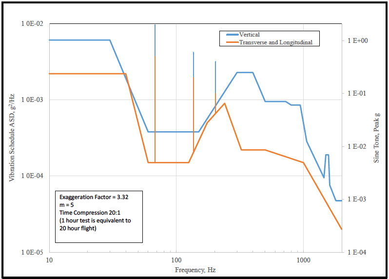
Figure description:
Vibration Schedule ASD and Sine Tone versus Frequency
Vibration Schedule
Legend
- Vertical — color: blue; symbol: Solid line with markers
- Transverse and Longitudinal — color: orange; symbol: Solid line with markers
| Frequency (Hz) | Vertical ASD (g²/Hz) | Transverse and Longitudinal ASD (g²/Hz) | Vertical Sine Tone (Peak g) | Transverse and Longitudinal Sine Tone (Peak g) |
|---|---|---|---|---|
| 10 | 6.0E-03 | 2.2E-03 | null | null |
| 30 | 6.0E-03 | 2.2E-03 | null | null |
| 40 | 3.5E-03 | 2.2E-03 | null | null |
| 60 | 4.0E-04 | 1.5E-04 | null | null |
| 68 | 4.0E-04 | 1.5E-04 | 1.0E+00 | 4.0E-01 |
| 130 | 4.0E-04 | 1.5E-04 | null | null |
| 145 | 4.0E-04 | 1.9E-04 | 5.0E-01 | 2.0E-01 |
| 160 | 4.0E-04 | 2.5E-04 | null | null |
| 215 | 7.0E-04 | 6.5E-04 | 3.0E-01 | 1.2E-01 |
| 250 | 9.0E-04 | 9.0E-04 | null | null |
| 350 | 2.5E-03 | 2.2E-04 | null | null |
| 450 | 2.5E-03 | 2.2E-04 | null | null |
| 550 | 9.5E-04 | 2.2E-04 | null | null |
| 750 | 9.5E-04 | 1.8E-04 | null | null |
| 780 | 8.5E-04 | 1.7E-04 | null | null |
| 950 | 8.5E-04 | 1.6E-04 | null | null |
| 1000 | 5.0E-04 | 1.5E-04 | null | null |
| 1100 | 2.8E-04 | 1.2E-04 | null | null |
| 1450 | 9.5E-05 | 5.5E-05 | null | null |
| 1550 | 2.0E-04 | 4.5E-05 | null | null |
| 1650 | 2.0E-04 | 3.5E-05 | null | null |
| 1750 | 7.0E-05 | 3.0E-05 | null | null |
| 2000 | 5.0E-05 | 2.5E-05 | null | null |
Notes: Exaggeration Factor = 3.32 m = 5 Time Compression 20:1 (1 hour test is equivalent to 20 hour flight
Figure 514.8C-11. Category 8 - Propeller aircraft vibration exposure, 4-bladed C-130.
| Vertical Axis Broadband Random | Vertical Axis Sinusoidal Components | Longitudinal and Transverse Broadband Random | |||
|---|---|---|---|---|---|
| Frequency, Hz | ASD, g²/Hz | Center Frequency, Hz (Blade Order) | Acceleration peak (gpk) | Frequency, Hz | ASD, g²/Hz |
| 10 | 0.0032 | 17 (R) | 0.5 | 10 | 0.0022 |
| 30 | 0.0032 | 68 (nR) | 2 | 40 | 0.0022 |
| 60 | 0.0002 | 136(2nR) | 0.6 | 60 | 0.00015 |
| 150 | 0.0002 | 204 (3nR) | 0.4 | 125 | 0.00015 |
| 300 | 0.0012 | Overall rms, g | 1.76 | 175 | 0.0005 |
| 400 | 0.0012 | 240 | 0.0009 | ||
| 500 | 0.0005 | 325 | 0.00022 | ||
| 725 | 0.0005 | 500 | 0.00022 | ||
| 800 | 0.00045 | 1000 | 0.00015 | ||
| 943 | 0.00045 | Longitudinal and Transverse Sinusoidal Components | 2000 | 0.00002 | |
| 1061 | 0.00015 | rms, g | 0.61 | ||
| 1450 | 0.00005 | Center Frequency, Hz (Blade Order) | Acceleration peak (gpk) | ||
| 1500 | 0.0001 | ||||
| 1575 | 0.0001 | 17 (R) | 0.2 | ||
| 1610 | 0.00004 | 68 (nR) | 0.5 | ||
| 1800 | 0.000025 | 136 (2nR) | 0.2 | ||
| 2000 | 0.000025 | 204 (3nR) | 0.1 | ||
| rms, g | 0.84 | Overall rms, g | 0.74 | ||
| Test Duration per axis: 1 hour for 20 hours of flight. | |||||
MIL-STD-810H
METHOD 514.8, ANNEX C
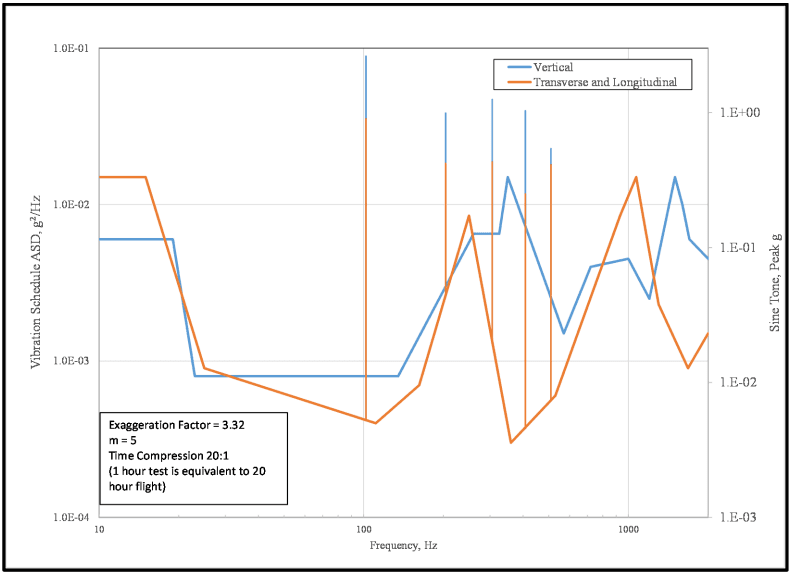
Figure description:
Vibration Specification Chart with Dual Y-Axes, Frequency and ASD/Sine Tone Data
Vibration Schedule ASD and Sine Tone peak g
Legend
- Vertical — color: blue; symbol: solid line with vertical spikes
- Transverse and Longitudinal — color: orange; symbol: solid line with vertical spikes
Annotations
- Exaggeration Factor = 3.32 (text_label - position: bottom-left box)
- m = 5 (text_label - position: bottom-left box)
- Time Compression 20:1 (text_label - position: bottom-left box)
- (1 hour test is equivalent to 20 hour flight (text_label - position: bottom-left box))
| Frequency (Hz) | Vertical ASD (g²/Hz) | Transverse and Longitudinal ASD (g²/Hz) | Vertical Sine Tone (Peak g) | Transverse and Longitudinal Sine Tone (Peak g) |
|---|---|---|---|---|
| 10 | 6.0E-03 | 1.5E-02 | ||
| 16 | 1.5E-02 | |||
| 20 | 6.0E-03 | 6.0E-03 | ||
| 25 | 8.0E-04 | 9.0E-04 | ||
| 102 | 9.0E-01 | 1.2E-01 | ||
| 115 | 4.0E-04 | |||
| 140 | 8.0E-04 | |||
| 170 | 7.0E-04 | |||
| 225 | 4.0E-01 | 1.5E-01 | ||
| 250 | 8.5E-03 | |||
| 300 | 6.5E-03 | 1.2E-03 | ||
| 350 | 5.0E-01 | 2.0E-01 | ||
| 400 | 6.5E-03 | 3.0E-04 | ||
| 420 | 1.5E-02 | |||
| 440 | 2.0E-01 | 5.0E-02 | ||
| 520 | 3.0E-01 | 1.5E-01 | ||
| 550 | 6.0E-04 | |||
| 600 | 1.5E-03 | |||
| 660 | 1.5E-01 | 1.0E-01 | ||
| 750 | 4.0E-03 | |||
| 1000 | 4.5E-03 | |||
| 1100 | 1.5E-02 | |||
| 1200 | 2.5E-03 | |||
| 1400 | 2.5E-03 | |||
| 1600 | 1.5E-02 | |||
| 1750 | 9.0E-04 | |||
| 1850 | 6.0E-03 | |||
| 2000 | 4.5E-03 | 1.5E-03 |
Figure 514.8C-12. Category 8 - Propeller aircraft vibration exposure. 6-bladed C-130
| Vertical Axis Broadband Random | Vertical Axis Sinusoidal Components | Longitudinal and Transverse Broadband Random | |||
|---|---|---|---|---|---|
| Frequency, Hz | ASD, g²/Hz | Center Frequency, Hz (Blade Order) | Acceleration peak (gpk) | Frequency, Hz | ASD, g²/Hz |
| 10 | 0.006 | 102 (nR) | 2.62 | 10 | 0.015 |
| 19 | 0.006 | 204 (2nR) | 0.99 | 15 | 0.015 |
| 23 | 0.0008 | 306 (3nR) | 1.25 | 25 | 0.0009 |
| 135 | 0.0008 | 408 (4nR) | 1.03 | 111 | 0.0004 |
| 260 | 0.0065 | 510 (5nR) | 0.54 | 162 | 0.0007 |
| 325 | 0.0065 | Overall rms, g | 3.97 | 250 | 0.0085 |
| 350 | 0.015 | 360 | 0.0003 | ||
| 570 | 0.0015 | 530 | 0.0006 | ||
| 720 | 0.004 | Longitudinal and Transverse | 930 | 0.0085 | |
| 1000 | 0.0045 | Sinusoidal Components | 1070 | 0.015 | |
| 1200 | 0.0025 | Center Frequency, Hz (Blade Order) | Acceleration peak (gpk) | 1300 | 0.0023 |
| 1500 | 0.015 | 1680 | 0.0009 | ||
| 1600 | 0.01 | 102 (nR) | 0.9 | 2000 | 0.0015 |
| 1700 | 0.006 | 204 (2nR) | 0.42 | rms, g | 2.49 |
| 2000 | 0.0045 | 306 (3nR) | 0.43 | ||
| rms, g | 3.22 | 408 (4nR) | 0.25 | ||
| 510 (5nR) | 0.41 | ||||
| Overall rms, g | 2.63 | ||||
| Test Duration per axis: 1 hour for 20 hours of flight. | |||||
MIL-STD-810H
METHOD 514.8, ANNEX C
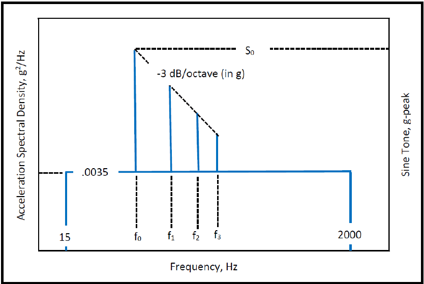
Figure description:
Composite Vibration Spectrum
Acceleration Spectral Density and Sine Tone Profile
Annotations
- S₀ (text_label - position: Peak level of the sine tone at frequency f₀)
- .0035 (text_label - position: Constant level of the Acceleration Spectral Density floor)
- -3 dB/octave (in g (text_label - position: Slope connecting the peaks of the sine tones at f₀, f₁, f₂, and f₃))
| Frequency (Hz) | Acceleration Spectral Density (g²/Hz) | Sine Tone (g-peak) |
|---|---|---|
| 15 | 0.0035 | null |
| f₀ | 0.0035 | S₀ |
| f₁ | 0.0035 | S₁ |
| f₂ | 0.0035 | S₂ |
| f₃ | 0.0035 | S₃ |
| 2000 | 0.0035 | null |
Notes: The chart displays a dual-axis vibration profile. The left y-axis represents Acceleration Spectral Density (g²/Hz for the random vibration floor, which is constant at 0.0035 g²/Hz between 15 Hz and 2000 Hz. The right y-axis represents the level of discrete Sine Tones (g-peak superimposed on the random background at frequencies f₀, f₁, f₂, and f₃. The peak levels of these sine tones decrease following a slope of -3 dB per octave starting from S₀ at f₀.))
Figure 514.8C-13. Category 8 - Propeller aircraft vibration exposure. Other than C-130
| TRANSPORTATION LOCATIONS (see Figure 514.8C-14) | NARROWBAND LEVEL L0 (g2/Hz) |
|---|---|
| In fuselage forward of propeller | 0.035 |
| In fuselage within one propeller blade radius of propeller passage plane | 0.42 |
| In fuselage or wing aft of propeller | 0.11 |
| 1/ f0 = blade passage frequency (propeller rpm times number of blades) (Hz). f1 = 2 × f0 f2 = 3 × f0 f3 = 4 × f0 | |
| 2/ Test should be conducted as sine-on-random, with: S0 = 1.414 * √0.1 * f0 * L0 | |
| 3/ Sine tones may be swept to account for known variance in blade passing frequency. | |
| 4/ If transportation location is unknown test to highest S0 level of the possible locations. | |
| 5/ Test duration per axis: 1 hour for 20 hours of flight. | |
| 6/ The broadband and narrowband levels were derived from previous versions of this standard by decompression from 1000 to 20 flight hours per hour runtime utilizing Equation 9.5 of Annex F with m = 7.5 (slope for acceleration spectral density). | |
MIL-STD-810H METHOD 514.8, ANNEX C
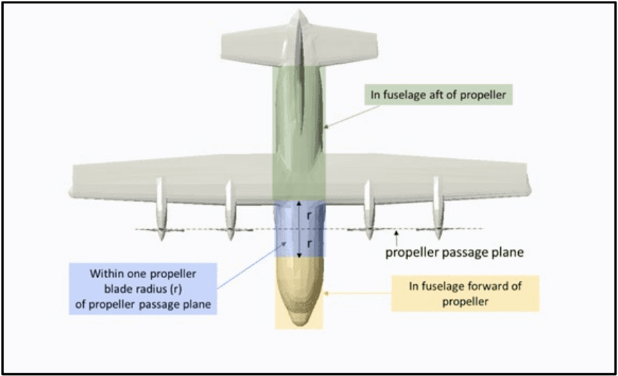
Figure description:
- Subject: Propeller aircraft transportation locations (excluding C-130 per MIL-STD-810H.
- Key Reference: Propeller passage plane (dashed line through propeller hubs.
- Transportation Zones:
- In fuselage forward of propeller: Yellow shaded area at the nose.
- Within one propeller blade radius (r of propeller passage plane: Blue shaded band extending distance 'r' both forward and aft of the propeller passage plane.
- In fuselage aft of propeller: Green shaded area covering the mid-to-rear fuselage.
Figure 514.8C-14. Category 8 - Propeller aircraft transportation locations (other than C-130).
514.8-2.5 Category 16 - Aircraft stores - materiel, jet aircraft
Materiel installed within a jet aircraft store will experience the store vibration discussed in paragraph 2.4. The input exposure levels for materiel within the store are essentially the same as response levels of the store. If gunfire, cavity resonance, buffet-maneuver, and free-flight conditions occur for the store, the materiel will also be exposed to these conditions.
- a. Exposure levels. Base vibration criteria on in-flight measurements when possible. If satisfactory flight measurements are not available, derive levels from Table 514.8D-IV and Figure 514.8D-9.
Note: Use input control for vibration testing of this materiel rather than response control (see paragraph 4.2.1 in the front part of this Method).
- b. Exposure durations. Take durations from the Life Cycle Environment Profile.
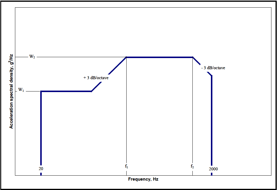
Figure description:
Random Vibration Test Profile Envelope
Acceleration spectral density vs Frequency
Annotations
- + 3 dB/octave (text_label - position: Slope of the segment between the W1 plateau and f1)
- - 3 dB/octave (text_label - position: Slope of the segment starting at f2)
- W1 (text_label - position: First horizontal plateau level on y-axis)
- W2 (text_label - position: Second horizontal plateau level on y-axis)
- f1 (vertical_line - position: Frequency at the start of the W2 plateau)
- f2 (vertical_line - position: Frequency at the end of the W2 plateau)
| Frequency (Hz) | Acceleration spectral density (g²/Hz) |
|---|---|
| 20 | 0 |
| 20 | W1 |
| [unlabeled | W1 |
| f1 | W2 |
| f2 | W2 |
| 2000 | [unlabeled |
| 2000 | 0 |
Notes: The graph depicts a standard random vibration power spectral density (PSD envelope. It defines level plateaus (W1, W2 and sloped segments (+3 dB/octave and -3 dB/octave between specified frequency points (20 Hz, f1, f2, and 2000 Hz.))))
Figure 514.8D-9. Category 16 - Jet aircraft store equipment vibration exposure.
514.8-2.5 DFL – Upper Distribution-Free Tolerance Limit
The distribution-free tolerance limit that uses the original untransformed sample values is defined to be the upper limit for which at least the fraction of all sample values will be less than the maximum predicted or measured value with a confidence coefficient of " ". This limit is based on order statistic considerations.
where is the maximum value of the set of estimates, , is the fractional proportion below , and is the confidence coefficient. , and are not independently selectable. That is
- (1) Given and assuming a value of , the confidence coefficient can be determined.
(2) Given and , the proportion can be determined.
- (3) Given and , the number of samples can be determined such that the proportion and confidence can be satisfied (for statistical experiment design).
may not be meaningful for small samples of data, , and comparatively large , . is sensitive to the estimate bandwidth.
514.8-2.5 Spectral spike Removal (Step 5)
For combined SOR or NBROR environments, the sine tones or narrowbands must be processed separately from the broadband random. Step 5 provides a method of removing the sine tones or narrowbands from the ASD(Sum) spectra when required.
To insure accuracy and to isolate unexpected inconsistencies in the data, the spectral spikes are selected and removed by the analyst acting interactively in a program loop using a graphical interface such as that shown in Figure 514.8F- D.2. The analyst selects the beginning and ending frequency of all spectral spikes for which removal is desired. Intermediate points are then replaced with a logarithmic interpolation of the two endpoints to produce the broadband ASD(SpkRmvd), shown as magenta in Figure 514.8F-D.2. This is the fifth ASD of the single-event ASD sum-set and becomes the working ASD for the broadband profile development.
Note that the width of the spectral spikes removed will depend on a number of factors, including, but not limited to, the nature of the data and the frequency resolution of the ASD calculations. Typically, the data should be pre-processed to determine if the data is more narrowband random or more sinusoidal in nature. This information determines how the narrow-band energy will be processed.
MIL-STD-810H
METHOD 514.8, ANNEX F, APPENDIX D
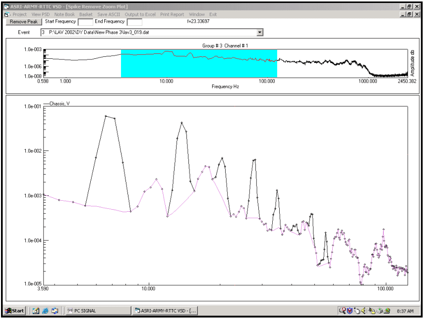
Figure description:
Spectral Analysis and Spike Removal Zoom Plot Event 3: P:\LAV 2002\DY Data\New Phase 3\lav3_019.dat
Group # 3 Channel # 1
Annotations
- Selected Frequency Range for Zoom (shaded_area - position: x from 3.590 to 100.000)
| Frequency (Hz) | Amplitude (Overview) |
|---|---|
| 0.598 | 1.0e-005 |
| 1.0 | 5.0e-006 |
| 10.0 | 5.0e-004 |
| 100.0 | 5.0e-005 |
| 1000.0 | 1.0e-007 |
| 2450.382 | 1.0e-008 |
Spike Remove Zoom Plot
Legend
- Chassis, V — color: black; symbol: line with diamonds
- De-spiked (implied — color: purple; symbol: line with diamonds
| Frequency (Hz) | Chassis, V (Black) | Processed/De-spiked (Purple) |
|---|---|---|
| 3.590 | 1.0e-003 | 1.0e-003 |
| 4.0 | 8.0e-004 | 8.0e-004 |
| 5.0 | 6.0e-004 | 6.0e-004 |
| 6.0 | 4.0e-002 | 5.0e-004 |
| 6.5 | 6.0e-002 | 4.5e-004 |
| 7.5 | 5.0e-002 | 4.8e-004 |
| 8.5 | 6.0e-004 | 6.0e-004 |
| 10.0 | 1.5e-003 | 1.5e-003 |
| 11.0 | 2.5e-003 | 2.5e-003 |
| 13.0 | 1.0e-003 | 1.0e-003 |
| 15.0 | 1.5e-003 | 4.5e-004 |
| 16.5 | 4.0e-002 | 6.5e-004 |
| 18.0 | 2.5e-002 | 9.0e-004 |
| 20.0 | 1.5e-003 | 1.5e-003 |
| 25.0 | 4.5e-003 | 4.5e-003 |
| 33.0 | 5.0e-003 | 6.0e-004 |
| 37.0 | 7.0e-003 | 4.0e-004 |
| 45.0 | 5.0e-004 | 3.5e-004 |
| 52.0 | 6.5e-003 | 3.2e-004 |
| 65.0 | 1.3e-003 | 1.8e-004 |
| 85.0 | 1.0e-004 | 1.0e-004 |
| 100.0 | 1.8e-004 | 1.8e-004 |
Source: ASRI-ARMY-RTTC VSD Notes: The software interface indicates a spike removal process being performed on a spectral data file (lav3_019.dat. The top plot provides a wide frequency context, while the bottom plot is a detailed log-log view of the highlighted 3.59Hz - 100Hz region. Current cursor frequency f=23.33697 is noted in the header.)
Figure 514.8F-D.2. Spectral spike removal window.
The nature of the vibration is dependent upon the vehicle and field environment. For example, an item mounted on a wheeled vehicle and driven on primary (paved) roads will be exposed to a broadband random forcing function. A wheeled vehicle driven over a periodic washboard course will typically produce a combined SOR vibration environment, as will a rotary wing aircraft. A tracked vehicle usually produces a combined NBROR vibration. The nature of the data (sine or narrorband) needs to be determined at this point. Refer to Annex F, paragraph 4 for more discussion on the nature of the vibration. Although the frequency resolution selected for ASD calculations will affect the width and amplitude of spectral spikes, it will not affect the total g-rms of the spectral spikes removed. For that reason the g-rms of the spectral spikes, rather than the ASD amplitude, should be used when processing the narrowband information.
The energy corresponding to the removed spectral spikes can be exported in a form that facilitates spreadsheet analysis. This allows external processing of the narrowband energy. Two spreadsheets should be produced. One containing the center frequency, width, and the total g-rms of all spectral spikes removed from all ASD(Sum); and another containing the same information from all ASD(Avg). The average numbers are used for SOR developments while the sum numbers are used for NBROR developments. The procedures used to process the narrowband information are presented in paragraph 3.
An example spectral spike removed spreadsheet is provided in Table 514.8F-D.III. The example contains the energies removed from the ASD(Avg). The ASD(Sum) table is identical except the g-rms levels are derived from the ASD(Sum) instead of the ASD(Avg). This particular example is of a wheeled vehicle on a two-inch wasboard course. Note that the fundamental and two additional harmonics were removed from each of three events (5, 7.5, and 10 mph 2” wasboard).
MIL-STD-810H
METHOD 514.8, ANNEX F, APPENDIX D
| Project File: | Example Wheeled Vehicle | [ ] | |||||
|---|---|---|---|---|---|---|---|
| Total Miles: | 1000 | Block size : | 4096 | Start Freq: 3 | Raw ASD | W-UCol ASD | |
| Date Proc :9/16/2002 | Window Type: | Hann | End Frq: 500 | N: | 1 | 1 | |
| Time Proc :6:37:44 AM | Min g-rms: | 0.5 | Rmv DC : Y | M: | 2 | 2 | |
| Total G-RMS of removed Spectral spike | |||||||
| Channel | 1 | 2 | 3 | ||||
| Description | Channel 1 | Channel 2 | Channel 3 | ||||
| Type | ASD(Avg) | ASD(Avg)| | ASD(Avg) | ||||
| Test Time | 30 | 30 | 30 | ||||
| Event | Beta Dist Time | Center Freq | Bandwidth Selected | g-rms | g-rms | g-rms | |
| 1 Harmonic | 5 mph 2" WB | 8.31 | 3.67 | 6 | 0.1534 | 2.79E-02 | 5.31E-02 |
| 7.5 mph 2" WB | 21.28 | 5.50 | 5 | 0.2691 | 3.41E-02 | 0.134565 | |
| 10 mph 2" WB | 7.47 | 7.33 | 7 | 0.5755 | 8.74E-02 | 0.5730498 | |
| 2 Harmonic | 5 mph 2" WB | 8.31 | 7.33 | 6 | 0.1118 | 3.49E-02 | 7.37E-02 |
| 7.5 mph 2" WB | 21.28 | 11.00 | 7 | 8.72E-02 | 3.22E-02 | 5.18E-02 | |
| 10 mph 2" WB | 7.47 | 14.67 | 6 | 8.98E-02 | 2.67E-02 | 0.211421 | |
| 3 Harmonic | 5 mph 2" WB | 8.31 | 11.00 | 6 | 0.06546 | 4.01E-02 | 9.12E-02 |
| 7.5 mph 2" WB | 21.28 | 16.50 | 9 | 2.63E-02 | 2.94E-02 | 0.05846 | |
| 10 mph 2" WB | 7.47 | 22.00 | 8 | 3.08E-02 | 3.75E-02 | 0.07558 | |
2.5.1 Modal test techniques
Experimental modal tests involve excitation of a structure with a measured force while measuring the acceleration response and computing the frequency response functions (FRF) at location(s) of interest for subsequent modal analysis. Excitation of the structure for modal test may be accomplished in various ways. The simplest method, a modal impact test, consists of excitation with a modally tuned impact hammer instrumented with a force gage to produce a low force impact on the structure that approximates an impulse function. This technique is commonly used as a quick check of resonant frequencies for fixtures and installed components. A more sophisticated approach would use burst random excitation with small vibration exciter(s) attached to a structure that is instrumented with an array of accelerometers. Modal tests with vibration exciters is more commonly used for high channel count modal tests of complex structures with more precise measurements required for the development of mode shapes and verification of analytical models. Sinusoidal and broadband random vibration excitation of a test fixture/item mounted on large vibration exciters are also options to check resonant frequencies for laboratory vibration test setups. Select methodology that will result in well-understood, usable data, and that will provide the level or detail needed for the specific test goals.
2.5.2 Material non-linear behavior
Dynamic inputs should be at as realistic levels as possible, and at as many levels as practical because materiel response is generally nonlinear with amplitude. Modal parameters determined through modal test and analysis techniques are typically based on assumption of structural linearity. Linearity checks can be conducted during modal tests by collecting and analyzing data at various force levels and identifying frequency shifts, if any, in the resonant frequencies. For structures that exhibit highly non-linear behavior, additional analysis will be required to extrapolate modal test results to the expected life cycle vibration environments.
2.6 Aerodynamic Effects
A primary source of vibration in aircraft and aircraft stores is the aerodynamic flow over the vehicle. Oscillating pressures (turbulence) within the flow drive vibration of the airframe surfaces. These pressures and, thus, the vibration are a linear function of dynamic pressure, and a non-linear function of Mach number. When a flow becomes supersonic, it smooths out and turbulence drops off. Then, as speed increases, further turbulence builds up again. This phenomenon is well illustrated in the vibration data contained in paragraph 6.1, reference k. The Mach corrections given in Annex D, Table 514.8D-IV are based on an average of this data. The following definitions and the values and the formulas of Annex D, Table 514.8D-V are provided for use in calculating airspeeds and dynamic pressures. The source of the formulas is paragraph 6.1, reference ff, and the source of the atmospheric values is paragraph 6.1, reference kk.
514.8-2.6 Category 9 - Aircraft - helicopter
- a. Environment characterization. Vibration of cargo carried in helicopters is characterized by a continuous wideband, low-level background with strong narrowband peaks superimposed. This environment is a combination of many sinusoidal or near sinusoidal components due to main and tail rotors, rotating machinery and low-level random components due to aerodynamic flow. These sources are discussed in Annex D, paragraph 2.3.
Data acquired from variants of the rotorcraft listed in Table 514.8C-XIVa, were used to develop the random levels, source frequency relationships, and peak acceleration relationships reported in Table 514.8C-XIVb. Aircraft specific source frequencies are directly associated with rotor blade count and rotation speed. Tabulated source frequency ranges, peak acceleration amplitudes and associated random levels were empirically determined and encompass the vibration environments measured. The suitability of extrapolating these empirical peak acceleration relationships to aircraft not listed is unknown. Application of these empirical relationships to rotorcraft that are not included in the sample set should be applied with caution and only in the total absence of field data. Whenever possible, vehicle specific flight data should be acquired and employed in development of an aircraft specific vibration criterion.
-
b. Sling loads. Cargo carried as sling loads below a helicopter is normally subjected to low level random vibration due to turbulent flow around the cargo with narrow band peaks due to helicopter main rotor blade passage. In addition, there will be low frequency (primarily vertical) motions due to the sling suspension modes (similar to vibration isolator modes, see Annex A, paragraph 2.4.2). Choose slings based on sling stiffness and suspended mass such that suspension frequencies (fs) do not coincide with helicopter main rotor forcing frequencies (fi). Ensure suspension frequencies are not within a factor of two of forcing frequencies (fs < fi / 2 or fs > 2 fi). Determine main rotor forcing frequencies (shaft rotation frequency, blade passage frequency, and harmonics) for several helicopters from Table 514.8C-XIV. When inappropriate combinations of cargo and slings are used, violent vibration can occur. The cargo is likely to be dropped to protect the helicopter.
-
c. Exposure levels.
-
(1) Helicopter internal cargo vibration is a complex function of location within the helicopter cargo bay and the interaction of the cargo mass and stiffness with the helicopter structure. Measurements of the vibration of the cargo in the specific helicopter are necessary to determine vibration with any accuracy. Approximate criteria may be derived from Annex D, paragraph 2.3. These levels are intended to envelope potential worst-case environments, and have been aggressively compressed in time. Additional tailored helicopter vibration schedules are provided in TOP 01-2-603 paragraph 6.1, reference xx.
NOTE: These levels are intended to envelope potential worst-case environments, and have been aggressively compressed in time (paragraph 6.1, reference ww indicates a time compression from 2500 hours to 4 hours using the equation shown in paragraph 2.3f with a value of m=6). They do not represent environments under which vibration-sensitive materiel should be expected to perform to specification. However, the materiel is expected to survive undamaged, and to function to specification at the completion of the test.
- (2) Slung cargo levels are low and should not be a significant factor in design of materiel that has a reasonable degree of ruggedness.
- (3) Plans for development of updated vibration schedules representative of the modern rotorcraft fleet are in progress. As each aircraft’s vibration schedule updates are completed, they will be provided as individual Annexes to TOP 01-2-603 (Rotorcraft Laboratory Vibration Test Schedules) along with vibration schedule development (VSD) technique details and all relevant descriptors such as mission scenario and instrumentation locations. The updated schedules will supersede the current defaults as listed in Table 514.8C-XIV. Currently there are only two rotorcraft in TOP 01-2-603, the UH-60 and the CH-47. These helicopters have therefore been removed from Table 514.8C-XIV.
- d. Exposure durations. When measured data are used to establish exposure levels, take durations from the LCEP. Otherwise refer to the guidance provided in paragraph 2.3d in Annex D of this method.
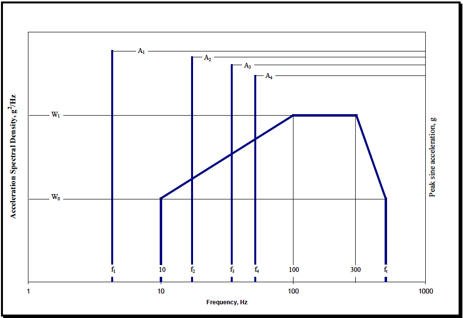
Figure description:
Vibration Specification Chart
Combined Random and Sine Vibration Profile
Annotations
- W1 (horizontal_line - position: left y-axis level W1)
- W0 (horizontal_line - position: left y-axis level W0)
- A1 (horizontal_line - position: right y-axis level A1)
- A2 (horizontal_line - position: right y-axis level A2)
- A3 (horizontal_line - position: right y-axis level A3)
- A4 (horizontal_line - position: right y-axis level A4)
| Frequency (Hz) | Acceleration Spectral Density (g²/Hz) | Peak sine acceleration (g) |
|---|---|---|
| f1 | null | A1 |
| 10 | W0 | null |
| f2 | null | A2 |
| f3 | null | A3 |
| f4 | null | A4 |
| 100 | W1 | null |
| 300 | W1 | null |
| ft | W0 | null |
Notes: The chart illustrates a composite vibration test specification. The thick blue line represents the random vibration profile defined in terms of Acceleration Spectral Density (g²/Hz with key levels W0 and W1. The thin blue vertical lines represent discrete sine vibration components (sine peaks at frequencies f1, f2, f3, and f4 with corresponding peak acceleration amplitudes A1, A2, A3, and A4. The x-axis is on a logarithmic scale from 1 to 1000 Hz.))
Figure 514.8C-15. Category 9 - Helicopter vibration exposure. (Same as Annex D, Figure 514.8D-4.)
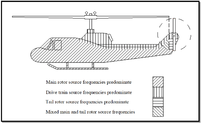
Figure description:
Key Entities and Information:
- Subject: Category 9 - Helicopter vibration zones.
- Main Rotor Source Frequencies: Predominate in the main fuselage and cockpit area (indicated by diagonal lines slanting down to the right.
- Drive Train Source Frequencies: Predominate in the upper section of the fuselage near the main rotor mast (indicated by vertical lines.
- Tail Rotor Source Frequencies: Predominate in the immediate tail rotor assembly and rear vertical stabilizer (indicated by horizontal lines.
- Mixed Main and Tail Rotor Source Frequencies: Predominate along the tail boom (indicated by diagonal lines slanting down to the left.
Figure 514.8C-16. Category 9 - Helicopter vibration zones. (Same as Annex D, Figure 514.8D-5.)
MIL-STD-810H
METHOD 514.8, ANNEX C
| Helicopter | MAIN ROTOR | TAIL ROTOR | ||
|---|---|---|---|---|
| Rotation Speed 1P (Hz) | Number of Blades n | Rotation Speed 1T (Hz) | Number of Blades m | |
| AH-1 | 5.40 | 2 | 27.7 | 2 |
| AH-6J | 7.95 | 5 | 47.3 | 2 |
| AH-6M | 7.92 | 6 | 44.4 | 4 |
| AH-64 (early) | 4.82 | 4 | 23.4 | 4 |
| AH-64 (late) | 4.86 | 4 | 23.6 | 4 |
| CH-47D | Refer to TOP 01-2-603 (Paragraph 6.1, reference xx) | |||
| MH-6H | 7.80 | 5 | 47.5 | 2 |
| OH-6A | 8.10 | 4 | 51.8 | 2 |
| OH-58A/C | 5.90 | 2 | 43.8 | 2 |
| OH-58D | 6.60 | 4 | 39.7 | 2 |
| UH-1 | 5.40 | 2 | 27.7 | 2 |
| UH-60 | Refer to TOP 01-2-603 (Paragraph 6.1, reference xx) | |||
| MATERIEL | RANDOM LEVELS | SOURCE FREQUENCY (fx) RANGE (Hz) | PEAK ACCELERATION (Ax) at fx (GRAVITY UNITS (g)) |
|---|---|---|---|
| General | W0 = 0.0010 g²/Hz W1 = 0.010 g²/Hz ft = 500 Hz | 3 to 10 | 0.70/(10.70 - fx) |
| 10 to 25 | 0.10 x fx | ||
| 25 to 40 | 2.50 | ||
| 40 to 50 | 6.50 - 0.10 x fx | ||
| 50 to 500 | 1.50 | ||
| Instrument Panel | W0 = 0.0010 g²/Hz W1 = 0.010 g²/Hz ft = 500 Hz | 3 to ≤ 10 | 0.70/(10.70 - fx) |
| >10 to 25 | 0.070 x fx | ||
| 25 to 40 | 1.750 | ||
| 40 to 50 | 4.550 - 0.070 x fx | ||
| 50 to 500 | 1.050 | ||
| External Stores | W0 = 0.0020 g²/Hz W1 = 0.020 g²/Hz ft = 500 Hz | 3 to ≤ 10 | 0.70/(10.70 - fx) |
| >10 to 25 | 0.150 x fx | ||
| 25 to 40 | 3.750 | ||
| 40 to 50 | 9.750 - 0.150 x fx | ||
| 50 to 500 | 2.250 | ||
| On/Near Drive System Elements | W0 = 0.0020 g²/Hz | 5 to ≤ 50 | 0.10 x fx |
| W1 = 0.020 g²/Hz ft = 2000 Hz | > 50 to 2000 | 5.0 + 0.010 x fx |
| Main or Tail Rotor Frequencies (Hz) Determine 1P and 1T from the Specific Helicopter or from the table (below). | Drive Train Component Rotation Determine 1S from Specific Helicopter and Component. | |||
|---|---|---|---|---|
| f1 = 1P | f1 = 1T | f1 = 1S | ||
| f1 = 1P | f1 = 1T | fundamental | f1 = 1S | fundamental |
| f2 = n x 1P | f2 = m x 1T | blade passage (BP) | f2 = 2 x 1S | 2nd harmonic |
| f3 = 2 x n x 1P | f3 = 2 x m x 1T | 2nd harmonic | f3 = 3 x 1S | 3rd harmonic |
| f4 = 3 x n x 1P | f4 = 3 x m x 1T | 3rd harmonic | f4 = 4 x 1S | 4th harmonic |
514.8-2.6 Category 17 - Aircraft stores - assembled/materiel, propeller aircraft
There is no known source of general guidance or measured data for the vibration of propeller aircraft stores (except gunfire induced, see Method 519.8). However, since the excitation sources are the same, it seems likely that store vibration will be similar to that of the carrying aircraft. See paragraph 2.2 and Annex A, paragraph 2.3.3 for a discussion of this vibration. Maneuver buffet vibration experienced by stores of highly maneuverable propeller aircraft should be similar to that experienced by jet aircraft stores. See the buffet vibration portion of paragraph 2.4.1c.
- a. Exposure levels. There is no known source of data. For accurate definition of propeller aircraft store vibration, measurement of the actual environment is essential. The criteria of Table 514.8D-II and Figure 514.8D-2 may be used to develop preliminary estimates of general vibration. The criteria of Figure 514.8D-7 may be applied for maneuver buffet vibration.
- b. Exposure durations. Take durations from the Life Cycle Environment Profile (LCEP).
514.8-2.6 ETL – Upper Empirical Tolerance Limit
The empirical tolerance limit uses the original sample values and assumes the predicted or measured estimate set is composed of measurement points over frequency resolution bandwidths for a total of estimate values. That is
where is the average estimate at the frequency bandwidth over all measurement points
is used to construct an estimate set normalized over individual frequency resolution bandwidths. That is
where :
The normalized estimate set, , is ordered from smallest to largest and
where is the ordered element of set for
MIL-STD-810H METHOD 514.8, ANNEX F, APPENDIX B
is defined. For each resolution frequency bandwidth, then
Using implies that the value of at exceeds percent of the values with 50 percent confidence.
If a value other than is selected, the confidence level may increase. It is important that the set of estimates is homogeneous to use this limit, i.e., they have about the same spread in all frequency bands. In general, apply this limit only if the number of measurement points, , is greater than 10 .
514.8-2.6 Scenario Table (Step 6)
VSD requires knowledge of the exposure time for the individual events. For a ground vehicle, those times can be derived from the distribution of the system's mission scenario into the individual events through the use of a Beta distribution. For a helicopter, the scenario times are typically derived from the aircrafts usage spectrum. Further discussion of scenario development and the Beta distribution can be found in Annex F, paragraph 7.4.
The event times can be provided in the form of scenario tables populated in Step 6 of the process. An example scenario table is provided in Table 514.8F-D.IV. The weighting factors will be discussed further in paragraph 2.7. The example scenario table also includes a user input field for the slope to be used for time compression calculations. The remaining fields should be calculated by the software and contain the total g-rms levels of the ASD(SpkRmvd), over the user defined bandwidth of interest, for each channel of each event. For example, Column “1 GRMS” contains the g-rms levels for channel 1 for all events.
MIL-STD-810H
METHOD 514.8, ANNEX F, APPENDIX D Table 514.8F-D.IV. Scenario Table Input
| Event No | Event Name | Scenario Time | Weighted Factor Col | Weighted Factor Un-Col | 1 GRMS | 2 GRMS | 3 GRM |
|---|---|---|---|---|---|---|---|
| 1 | Radial Washboard 5 MPH | 6.62 | 1 | 6.62 | 0.0327 | 0.0639 | 0.06 |
| 2 | Radial Washboard 10 MPH | 9.76 | 1 | 9.76 | 0.0686 | 0.1309 | 0.19 |
| 3 | Radial Washboard 15 MPH | 3.51 | 1 | 3.51 | 0.1289 | 0.2524 | 0.30 |
| 4 | Embedded Rock 5 MPH | 9.01 | 1 | 9.01 | 0.0532 | 0.1201 | 0.12 |
| 5 | Embedded Rock 7.5 MPH | 11.04 | 1 | 11.04 | 0.0858 | 0.1839 | 0.18 |
| 6 | Embedded Rock 10 MPH | 4.74 | 1 | 4.74 | 0.1246 | 0.2647 | 0.22 |
| 7 | Belgian Block 5 MPH | 1.05 | 1 | 1.05 | 0.0238 | 0.0512 | 0.04 |
| 8 | Belgian Block 10 MPH | 3.24 | 1 | 3.24 | 0.0443 | 0.0862 | 0.08 |
| 9 | Belgian Block 15 MPH | 5.18 | 1 | 5.18 | 0.0616 | 0.1077 | 0.12 |
| 10 | Belgian Block 20 MPH | 5.02 | 1 | 5.02 | 0.0825 | 0.1542 | 0.16 |
| 11 | Belgian Block 25 MPH | 1.88 | 1 | 1.88 | 0.1238 | 0.2285 | 0.23 |
| Col Sum-Set GRMS | 0.1289 | 0.2647 | 0.300 | ||||
From this point forward, only the events with a g-rms above a threshold selected by the analyst will be processed. The threshold was presented in Table 514.8F-D.I (Minimum g-rms) and is set as a ratio of the maximum g-rms, typically 0.50. As higher level vibration dominates fatigue exposure, the exclusion of lower level events will have little effect on the final test time. When selecting the threshold for event inclusion, the analyst must consider both the preservation of the spectral information of the lower level events and the effects their shape will have on the more dominate, high level events. The events with a g-rms above the threshold will be referred to as “included events”.
For each channel, the software should calculate the peak and average g-rms of the included events. The average becomes the base g-rms level utilized for processing. The base g-rms level will be the g-rms of the vibration profiles before final adjustment of test times is made.
The primary function of Step 6 (Scenario Table) is to calculate a vibration runtime associated with each event. The calculations are made using Equation 9-5, a standard method based on the Miner-Palmgren hypothesis for adjusting vibration spectra test times and levels. The slope (m) is typically set to a value of 7.5 for broadband random calculations. Further discussions of Miner’s Rule can be found in Annex F, paragraph 9.0.
MIL-STD-810H
An example runtime table is provided in Table 514.8F-D.V. Individual events (1-11) are given in rows and individual channels (1-7) are given in columns. Table 514.8F-D.V has been populated by the software using equation 9-5 and the input provided in the Table 514.8F-D.IV. Note that the events for which the g-rms (given in Table 514.8F-D.IV) was less than 50 percent of the maximum g-rms (for the same channel) are set to a value of zero. For example, the maximum g-rms for channel 1 in Table 514.8F-D.IV is 0.1289 g-rms. Six of the eleven events have a g-rms greater than 0.0644 (0.5*0.1289) as reflected by the entries in Table 514.8F-D.V. The weighed-average g-rms of the six included events for channel 1 is 0.09198 g-rms. Application of Equation 9-5 for event 2 of channel 1, with G₁ = 0.0686 (from Table 514.8F-D.IV), G₂ = 0.09198 (the weighted-average g-rms), T₁ = 9.76 minutes (scenario time for event 2) yields a runtime for channel 1 and event 2 of T₂ = 1.0839, which is reflected in the entry of Table514.8F-D.V. The weighted rms is calculated by multiplying the scenario time by the associated g-rms. The weighted-average rms is the sum of the weighted g-rms values (for included events) divided by the sum of the scenario times (for included events). As all included events for a given channel are effectively normalized to the same g-rms level, the associated runtimes can simply be totaled to provide the overall runtime for that channel at that g-rms. The individual event run times are totaled in the row labeled TF in Table 514.8F-D.V. This total time is the run time required to provide equivalent broadband fatigue exposure to the system, assuming the broadband profile is also based on an average of the ASDs of the same group. The derivation of that average ASD will be discussed in paragraph 2.7.
| Event No | Event Name | Scenario Time | 1 (Min) | 2 (Min) | 3 (Min) | 4 (Min) | 5 (Min) | 6 (Min) | 7 (Min) |
|---|---|---|---|---|---|---|---|---|---|
| 1 | Radial Washboard 5 MPH | 6.62 | 0.0000 | 0.0000 | 0.0000 | 0.0000 | 0.0000 | 0.0000 | 0.000 |
| 2 | Radial Washboard 10 MPH | 9.76 | 1.0839 | 0.0000 | 7.5042 | 1.4266 | 0.0000 | 5.0242 | 0.000 |
| 3 | Radial Washboard 15 MPH | 3.51 | 44.0730 | 16.5723 | 67.7850 | 42.9182 | 31.0571 | 17.1557 | 33.406 |
| 4 | Embedded Rock 5 MPH | 9.01 | 0.0000 | 0.0000 | 0.0000 | 0.0000 | 0.0000 | 0.0000 | 0.648 |
| 5 | Embedded Rock 7.5 MPH | 11.04 | 6.5395 | 4.8474 | 4.7421 | 6.0680 | 3.1819 | 0.0000 | 21.373 |
| 6 | Embedded Rock 10 MPH | 4.74 | 46.1231 | 31.9828 | 10.4189 | 34.8946 | 6.6298 | 0.0000 | 38.806 |
| 7 | Belgian Block 5 MPH | 1.05 | 0.0000 | 0.0000 | 0.0000 | 0.0000 | 0.0000 | 0.0000 | 0.000 |
| 8 | Belgian Block 10 MPH | 3.24 | 0.0000 | 0.0000 | 0.0000 | 0.0000 | 0.0000 | 0.0000 | 0.000 |
| 9 | Belgian Block 15 MPH | 5.18 | 0.0000 | 0.0000 | 0.0000 | 0.0000 | 0.0000 | 0.0000 | 0.846 |
| 10 | Belgian Block 20 MPH | 5.02 | 2.2310 | 0.5887 | 0.9003 | 2.5947 | 3.1033 | 0.0000 | 2.898 |
| 11 | Belgian Block 25 MPH | 1.88 | 17.4201 | 4.2217 | 6.0418 | 16.9478 | 14.9296 | 0.0000 | 6.81 |
| TF | 117.4706 | 58.2131 | 97.3924 | 104.8499 | 58.9017 | 22.1799 | 104.791 | ||
| TFA | 60 | 30 | 60 | 30 | 30 | 15 |
MIL-STD-810H METHOD 514.8, ANNEX F, APPENDIX D
2.6.1 Dynamic pressure
The total pressure of a gas acting on an object moving through it is made up of static pressure plus dynamic pressure (q). The proportions vary with speed of the body through the gas. Dynamic pressure is related to speed by
q = 1/2 ρ V2 where ρ is the density of the gas, and V is the velocity of the object through the gas.
2.6.2 Airspeed
The speed of an aircraft moving through the atmosphere is measured in terms of airspeed or Mach number. There are several forms of airspeed designation that are discussed below. At sea level these are equal, but as altitude increases they diverge. Equations and data required for airspeed and dynamic pressure calculations are provided in Annex D, Table 514.8D-V. These are based on paragraph 6.1, references ff and kk.
- a. Calibrated airspeed. Airspeed is usually specified and measured in calibrated airspeed. Calibrated airspeed is typically expressed in nautical miles per hour (knots) and designated knots calibrated air speed (Kcas). Kcas is not true airspeed. It is derived from quantities that are directly measurable in flight. Since it is not true airspeed, it cannot be used in the simple formula for q given above.
MIL-STD-810H METHOD
2.6.3 Altitude
Aircraft air data systems measure local atmospheric pressure and convert this value to pressure altitude through a standard atmosphere model that relates pressure, temperature, and density. Pressure altitude is used in the equations relating airspeeds and dynamic pressure. Care must be exercised to assure that altitudes are pressure altitudes. Often, low altitude values for modern military aircraft are given as absolute height above local terrain. These values should be changed to pressure altitude values. Guidance from engineers familiar with mission profile development is required to make this adjustment.
2.7 Similarity
It is often desirable to use materiel in an application other than that for which it was developed. Also, changes are made to existing materiel or the environmental exposures because of an application change. The question arises as to how to verify that the materiel is suitable for the application? This is usually accomplished through a process called "qualification by similarity." Unfortunately, this process has never had a generally accepted definition. In practice it sometimes devolves to a paper exercise that provides traceability but has no engineering content. The following paragraphs are an adaptation of a set of criterion that was provided to an Air Force avionics program. It is suggested as a basis for vibration similarity criteria. Tailor the criteria for materiel type, platform environments, and program restraints. Change the emphasis from circuit cards to the particular critical elements when the materiel is not an electronic box. Also, change the fatigue equation exponents as appropriate.
514.8-2.7 Category 10 - Watercraft - Marine Vehicles
The vibration environment of cargo carried in ships is fundamentally the same as for materiel installed on ships. See Annex D, paragraph 2.10. For Navy vessels, see Method 528.1.
514.8-2.7 Category 18 - Aircraft stores - assembled/materiel, helicopter
Complex periodic waveforms characterize the service environment encountered by assembled stores externally carried on helicopters. Unlike stores carried on fixed-wing aircraft, externally mounted helicopter stores receive little aerodynamic excitation, particularly when compared with the rotor-induced vibration. Thus, most of the vibratory energy reaches the store and materiel through the attachment points between the aircraft and the store. Some excitation, however, is added along the entire store structure due to periodic rotor-induced pressure fluctuations. The result is a complex response, unique to the particular aircraft-store configuration. Therefore, realistic definition of the environment depends almost totally upon the use of in-flight vibration measurements. For stores exposed to gunfire, refer to Method 519.8.
- a. Exposure levels. Derive exposure levels for helicopter-carried store materiel from field measurements (paragraph 6.1, reference f contains criteria for specific helicopters). When measured data are not available, initial estimates can be derived from Table 514.8D-III, and Figures 514.8D-4 and 514.8D-5, prior to acquisition of field data. These levels are intended as worst-case environments and represent environments for which it may be difficult to develop vibration sensitive materiel. Materiel costs are often strongly influenced by the performance required in a vibration environment. Consequently, field measurement based vibration criteria are very important. To determine levels, locate the store relative to the helicopter zones as shown in Figure 514.8D-5. Most stores will be inside a vertical projection of the main rotor disc and should use the source frequencies of the main rotor in determining the values of A1, A2, A3, and A4 (see Table 514.8D-III). Also in Table 514.8D-III are the fundamental main rotor source frequencies of several helicopters.
- b. Exposure durations. When measured data are used to establish exposure levels, take durations from the LCEP. When levels are derived from Table 514.8D-III, and Figures 514.8D-4 and 514.8D-5, use a duration of four (4) hours in each of three (3) orthogonal axes for a total time of twelve (12) hours. This represents a 2500-hour operational life. Use the fatigue relationship of Annex A, paragraph 2.2 to trade test time for exposure level. Perform the calculation separately for each sinusoid and each segment of the broadband background.
514.8-2.7 Example from Measured Data
An example consisting of typical wheeled vehicle data (4 test courses, 3 data runs, 2 locations) is considered. The ensemble consists of a total of 24 average ASD measurements. The normal tolerance limit (NTL) of the 24 item ensemble (without being logarithm transformed) was computed as, as described in paragraph 2.4, and is illustrated in Figure 514.8F-B.2. For this example, and were selected, yielding a value of interpolated from Table 514.8F-B.I.
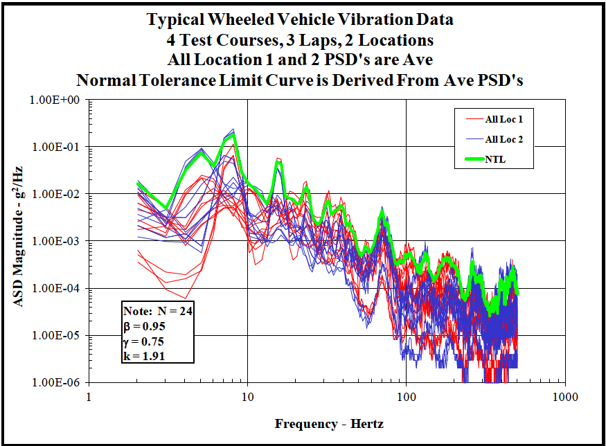
Figure description:
Typical Wheeled Vehicle Vibration Data 4 Test Courses, 3 Laps, 2 Locations
Typical Wheeled Vehicle Vibration Data
Legend
- All Loc 1 — color: red; symbol: Solid line
- All Loc 2 — color: blue; symbol: Solid line
- NTL — color: green; symbol: Thick solid line
| Frequency - Hertz | NTL (g²/Hz) | Loc 1 Envelope Range (g²/Hz) | Loc 2 Envelope Range (g²/Hz) |
|---|---|---|---|
| 2 | 1.70E-02 | 4.00E-04 - 9.00E-03 | 2.00E-03 - 1.50E-02 |
| 3 | 8.00E-03 | 1.00E-04 - 3.00E-03 | 1.00E-03 - 5.00E-03 |
| 4 | 5.00E-03 | 1.50E-04 - 3.00E-03 | 1.20E-03 - 4.00E-03 |
| 5 | 5.00E-02 | 2.00E-04 - 1.00E-02 | 2.00E-03 - 4.00E-02 |
| 7 | 1.00E-01 | 3.00E-02 - 6.00E-02 | 6.00E-02 - 1.20E-01 |
| 8 | 2.10E-01 | 4.00E-02 - 7.00E-02 | 8.00E-02 - 1.60E-01 |
| 10 | 1.80E-02 | 3.00E-03 - 8.00E-03 | 7.00E-03 - 1.50E-02 |
| 15 | 5.00E-02 | 5.00E-03 - 1.50E-02 | 1.00E-02 - 4.00E-02 |
| 20 | 1.00E-02 | 2.00E-03 - 5.00E-03 | 3.00E-03 - 8.00E-03 |
| 25 | 1.50E-02 | 2.00E-03 - 6.00E-03 | 4.00E-03 - 1.20E-02 |
| 35 | 7.00E-03 | 8.00E-04 - 3.00E-03 | 1.00E-03 - 5.00E-03 |
| 50 | 9.00E-04 | 2.00E-05 - 3.00E-04 | 5.00E-05 - 6.00E-04 |
| 70 | 5.00E-03 | 1.00E-04 - 1.50E-03 | 2.00E-04 - 4.00E-03 |
| 100 | 5.00E-04 | 1.00E-05 - 2.00E-04 | 2.00E-05 - 3.00E-04 |
| 150 | 7.00E-04 | 5.00E-06 - 2.00E-04 | 1.00E-05 - 5.00E-04 |
| 200 | 6.00E-04 | 1.00E-06 - 1.00E-04 | 3.00E-06 - 4.00E-04 |
| 300 | 2.00E-04 | 1.00E-06 - 8.00E-05 | 2.00E-06 - 1.50E-04 |
| 500 | 3.00E-04 | 1.00E-06 - 1.00E-04 | 2.00E-06 - 2.50E-04 |
Notes: All Location 1 and 2 PSD's are averages. Normal Tolerance Limit (NTL curve is derived from average PSDs. Statistical parameters provided: N = 24, ̠ = 0.95, ̡ = 0.75, k = 1.91.)
Figure 514.8F-B.2. Example normal tolerance limit applied to typical wheeled vehicle data.
MIL-STD-810H METHOD 514.8, ANNEX F, APPENDIX B
514.8-2.7 Calculate Weighted ASD (Step 7)
Steps 7 and 8 are used to complete the LVTS development process. At this point in the development process, an ensemble of single-event ASD sum-sets has been generated and consists of a sum-set for each channel of each event. The fifth ASD of the sum-set, the spectral spike removed ASD, is the working ASD for the VSD process. The multiple ASD(SpkRmvd) of a given channel (one for each event) must be combined to produce the broadband profile for that channel. The ASDs are combined using the methods discussed in the following paragraphs to produce a “group sumset”. The group sum-set, similar to the single-event ASD sum-set, includes a number of ASDs as defined in Table 514.8F-D.VI.
| ASD(Avg_g) | The weighted average of the ASD group. See Equation D.2-1. (See Ga(f) as defined in Appendix B) |
| ASD(Peak_g) | Calculated by holding the maximum amplitude of each spectral line over all events. |
| ASD(Stdv_g) | The weighted standard deviation of the ASD group. See Equation D2.2-3. (See Ge(f) as defined in Appendix B) |
| ASD(Sum_g) | Calculated by adding Ng standard deviations to the average for each spectral line. ASD(Sum_g) = Ng *ASD(Stdv_g) + ASD(Avg_g) Calculated by adding Ng standard deviations to the average for each spectral line. ASD(Sum) = Ng *ASD(Stdv) + ASD(Avg) Ng is a user defined variable typically set to 1. ASD(Sum) is limited by ASD(Peak) and Mg *ASD(Avg) where Mg is a user defined variable typically set to 2. (See Gf(f) as defined in Appendix B "for N=1") |
| ASD(Final) | The ASD(Sum_g) scaled to a user selected final time. |
The ASDs of the group sum-set, as with the single-event ASD sum-set, are calculated on a spectral line basis. The ASD(Avg_g) is an average of the ASD(SpkRmvd) for all events in the group (excluding those for which the g-rms is below the user defined threshold). Unlike the ASD(Avg) of the single-event ASD sum-set, the ASD(Avg_g) is not a standard n average ASD. Instead, the individual ASDs are weighted to the factors defined in the scenario table (see Table 514.8F-D.IV). Typically, the weighting factors are set equal to the individual event scenario times. The idea of a weighted approach is to produce a time-based calculation instead of an event-based calculation. In effect, weighting to the scenario time produces a separate ASD for each minute of the lifecycle, instead of an ASD for each event. Each minute of the system’s lifecycle would then be weighted equally in determining the average. A similar method is used to calculate the standard deviation of the group ASD(Stdv_g).
Assuming there are n events that exceed the minimum g-rms, that is weighting factor of each event, and that is the level of each event, then for each spectral line:
| ASD(Avg_g) = n ∑WiGi i=1 n ∑Wi i=1 | D.2-1 |
MIL-STD-810H METHOD 514.8, ANNEX F, APPENDIX D
D.2-2
The ASD(Sum_g) is calculated by adding N g standard deviations to the average, where N g is a user defined variable typically set to 1. Use of the ASD(Sum_g) is intended to account for factors such as differences in road surfaces, driver variances, and consideration of road surfaces not included in the data acquisition phase and other relevant variables. The ASD(Sum_g) is constrained to be no higher than M g *ASD(Avg_g) where M g is a user defined parameter with a default value of 2.0. The ASD(Sum_g) is also limited to the ASD(Peak_g) level at each spectral line. Although some additional processing may be required, the ASD(Sum_g) coupled with the runtime calculated in the previous step now represent the equivalent lifetime fatigue of an item mounted at that location. Recall that each channel represents a vibration axis for a given location. The ASD(Sum_g) becomes the working ASD and is passed forward to the next step.
In some cases multiple channels (or locations) must be combined into a single LVTS. This can be accomplished by simply enveloping the channels later in the VSD process. However, it is possible to combine multiple channels concurrently with the event combination. Assuming j is a list of m channels to combine, then for each spectral line:
D.2-3 D.2-4
2.7.1 Unmodified materiel
Qualify unmodified materiel by documented evidence that one of the following is met:
- a. The materiel was successfully qualified by test to vibration criteria that equals or exceeds the vibration requirements of the application.
- b. The materiel has demonstrated acceptable reliability in an application where vibration environments and exposure durations are equal to, or more stringent than the vibration requirements of the application.
- c. The materiel was successfully qualified by test to vibration criteria that falls short of the application ASD requirements in very narrow bands of energy (<5 percent of the test bandwidth) by no more than 3 dB, contingent that the materiel under test has no resonant frequencies within the subject narrow band, and that the G-rms falls within a minimum of 90 percent of the application and subsequently the materiel demonstrated acceptable reliability.
2.7.2 Modified materiel
Qualify modified materiel by documented evidence that the unmodified materiel meets the vibration requirements for the application supplemented by analyses and/or test data demonstrating that the modified materiel is dynamically similar to the unmodified materiel.
MIL-STD-810H METHOD
2.7.3 Equal vibration environment
Previous tests or other vibration exposures are considered to equal the application requirement when ALL of the following conditions are met:
- a. Previous exposures were the same type of vibration as the application requirement. That is, random vibration must be compared to random criteria, and sine must be compared to sine criteria.
- b. The exposure frequency range encompasses the application frequency range. Use a low frequency limit of the range that is the low frequency limit of the application requirement, or 1/2 of the lowest materiel resonant frequency, whichever is higher. The high frequency limit of the range is the high frequency limit of the application requirement.
- c. The exposure level (acceleration spectral density level or peak sinusoidal acceleration as applicable) was no more than 3.0 dB below the application requirement at any frequency, and was at or above the requirement for at least 80 percent of the total bandwidth.
- d. The fatigue damage potential of the exposure(s) is not less than 50 percent of the application fatigue damage potential at each frequency, and the fatigue damage potential of the exposure(s) equals or exceeds the application fatigue damage potential over 80 percent of the frequency range. State fatigue damage potentials as totaled equivalent exposure times at maximum application levels. Base summations and equivalencies on the relationships shown in paragraph 2.2 of this Annex. These relationships should be used with metal structures only.
2.7.4 Reliability data
Use field reliability data that meets all of the following criteria:
- a. The numbers of fielded materiel from which the data were taken are sufficient to statistically represent the specific materiel item.
- b. The field service seen by the materiel from which the data were taken is representative of the design environmental life cycle.
- c. The field reliability data satisfies maintainability, mission readiness, mission completion, and safety requirements.
2.7.5 Critical resonant response
Evaluate the first three natural frequencies of the chassis, and the first natural frequency of each sub assembly with the following procedure:
- a. Determine the required set (first set) of natural frequencies by test.
- b. Compare maximum levels at which the materiel is required to operate for the original qualification and for the application environment. Define the set (second set) of frequencies at which the application environment exceeds the original levels.
- c. Determine which resonances of the first set coincide with the frequencies of the second set. Show by test or analysis that the materiel will function as required when these resonances are exposed to the application environment maximum levels.
- d. Use the procedure of paragraph 2.2 above to compare the fatigue damage potential of the original qualification and the application environment. Define the set (third set) of frequencies at which the application fatigue damage potential exceeds the fatigue damage potential of the original criteria.
- e. Determine which resonances of the first set coincide with the frequencies of the third set. Show by test or analysis that the required materiel life will be obtained when these resonances are exposed to the application fatigue damage potential.
2.7.6 Dynamic similarity
Consider modified materiel as dynamically similar to baseline materiel when all of the following apply (circuit card used as an example):
MIL-STD-810H METHOD
2.8 Category 11 - Railroad - train
Cargo vibration levels for rail transport are generally low amplitude and have a moderately wide frequency bandwidth. The vibration levels can vary significantly with position on the railcar, load capacity, and track quality. Vertical axis vibration is typically the most severe followed by transverse and longitudinal. See Method 526.2, Rail Impact, for the shock associated with railcar longitudinal axis shock during coupling.
- a. Exposure levels. Transportation of non-isolated secured cargo on the railcar deck during cross country transportation is the typical environment. The ASD in Figure 514.8C-17 depicts the test severity at the railcar cargo deck. The vertical axis is up from the railcar deck, transverse is perpendicular across the rail tracks, and longitudinal is parallel to the rail tracks. The ASD is based on data measured the cargo deck of different railcars including flat cars, box cars, and refrigerated cars on US rail track. The data were collected from typical rail lines with track sections across switch yards, bridges, and track crossings. The data include a varying percentage of partial cargo load to maximum capacity, and a range of railcar speeds. The typical railcar average speed for the measurements is 80 - 96 km/hr (50 to 60 mph). The ASD is a worst case envelope of the measured data, time compressed to a test time of 12 hours representing 4,800 km
MIL-STD-810H
METHOD 514.8, ANNEX C
(3000 miles) of rail transport. The ASD is not representative of high-speed magnetic levitation suspension systems. The ASD also does not represent low frequency, transient displacement and shock typical in the transverse and longitudinal axes. Additional information on the ASD background is available in reference f.
- b. Exposure durations. Wheeled vehicle vibration amplitude is typically much higher than rail vibration and may eliminate the rail transportation test requirement. Rail vibration testing may be required for fragile or large mass equipment, or items shipped primarily by rail. Define the test duration based on the LCEP if the test is required. Measurements of the actual environment are recommended. If inadequate LCEP or field measurements are available use Figure 514.8C-17 to represent the worst case environment for each orthogonal axis. The default test duration is 12 hours/axis which represents 4,800 km (3,000 miles) of rail transport. An exaggeration factor of 1.5 using a value of m=7.5 (see paragraph 2.2 of Annex A for further explanation of exaggeration), is applied in Figure 514.8C-17.
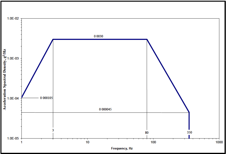
Figure description:
Annotations
- 0 000105 (text_label - position: y = 0.000105 at x = 1)
- 0 0030 (text_label - position: y = 0.0030 between x = 3 and x = 80)
- 0 000045 (text_label - position: y = 0.000045 at x = 350)
- 3 (vertical_line - position: x = 3)
- 80 (vertical_line - position: x = 80)
- 350 (vertical_line - position: x = 350)
| Frequency (Hz) | Acceleration Spectral Density (g²/Hz) |
|---|---|
| 1 | 0.000105 |
| 3 | 0.0030 |
| 80 | 0.0030 |
| 350 | 0.000045 |
| 350 | 0.0 |
Notes: The chart represents an acceleration spectral density profile on a log-log scale. The profile consists of a ramp-up from 1 to 3 Hz, a constant plateau from 3 to 80 Hz, and a ramp-down from 80 to 350 Hz, followed by a vertical drop at 350 Hz.
Figure 514.8C-17. Category 11 - Rail cargo vibration exposure.
MIL-STD-810H
METHOD 514.8, ANNEX D METHOD 514.8, ANNEX D Operational Tailoring Guidance for Vibration Exposure Definition
NOTE: Unless specifically noted, all document references refer to paragraph 6.1 of the front part of this Method.
514.8-2.8 Category 19 - Missiles - Tactical missiles (free flight)
There is no known source of general guidance or measured data for tactical missile carriage or launch vibration environments. Environments for jet aircraft, propeller aircraft, and helicopter carried missiles (stores) are discussed in paragraphs 2.4 through 2.7. Tactical carriage ground environments are discussed in paragraph 2.9. Free flight environments are covered in paragraphs 2.4.3 and 2.5 in regard to aircraft carried missiles. These environments should be generally applicable to tactical missiles during free flight mission segments.
- a. Exposure levels. There is no known source of data. For accurate definition of tactical missile free flight vibration, measurement of the actual environment is essential. The aircraft store criteria of Table 514.8D-IV and Figures 514.8D-6 and 514.8D-9 may be used to develop preliminary estimates of free flight vibration.
- b. Exposure durations. Take durations from the Life Cycle Environment Profile.
514.8-2.8 Calculate Weighted Intermediate LVTS (Step 8)
The next step in the development of the broadband vibration profile is to adjust the run time. The software should allow the analyst to select the runtime for each channel. In the example of Table 514.8F-D.V, the runtime for each channel is shown in the TFA field. Runtimes are typically adjusted to round the times calculated by the software to even time increments or to exaggerate the test schedule when desired. Care must be taken to assure the final LVTS levels do not overly exceed the maximum levels measured in the field and that exaggeration, if used, is not excessive. See Annex F, paragraph 9.2.1.2 for a discussion of limiting exaggeration. Step 8 simply applies Equation 9.5 to scale the ASD(Sum_g) to the user selected runtime, producing the final broadband ASD, ASD(Final).
Depending on the control methods used, further processing may be required. For SOR control the broadband profile must be combined with the sine tone information. It may also be necessary to combine the profiles of several channels into a single LVTS. At this point it is helpful to export the ASD(Final) in a form that facilitates spreadsheet analysis. This allows ease of processing for multi-channel combination, recombining with narrowband or sine tone, changes in runtime, or other specialized processing.
Note that an alternate method of combining the broadband profiles of multiple events into a representative LVTS is discussed in paragraph 7. This alternate method would begin with the ASD(SpkRmvd) and would produce an alternate ASD(Final).
MIL-STD-810H METHOD 514.8, ANNEX F, APPENDIX D
2.9 Category 20 - Ground vehicles - ground mobile. (See paragraph 6.1, references pp to vv.)
The ground mobile environment consists of broadband random vibration with peaks and notches. These peaks and notches are considerably higher and lower than the mean level. (See paragraph 6.1, reference d.) Terrain, road, and surface discontinuities, vehicle speed, loading, structural characteristics, and suspension system all affect this vibration. Gunfire criteria (Method 519.8) are not applicable since it is based on the response of aircraft-type structures that are significantly different than ground vehicle structures.
- a. Wheeled vehicles. There is presently no analytical model of these environments suitable for generalized application. A smooth spectrum similar to Annex C, Figure 514.8C-2 will be overly conservative at notches in the frequency spectrum. The spectra of Annex C, Figures 514.8C-4 through 514.8C-7 are typical of cargo bed responses in two-wheeled trailers and tactical wheeled vehicles (including four- wheeled trailers), respectively. This may be unrealistic for installed materiel since it does not consider vehicle structural response beyond the heavily supported cargo bed. The large assembly cargo test of Annex C, paragraph 2.3 can be adapted to provide highly accurate tests for this materiel.
MIL-STD-810H
METHOD 514.8, ANNEX D
- b. Tracked vehicles. The tracked vehicle environment is characterized by the strong influence of track patter that is related to the track pitch (length of a single track block) and the vehicle speed. The track induced component overlays a basic random environment similar to that discussed above for wheeled vehicles. This environment is best represented by superimposing narrowband random (track induced component) vibration at selected frequencies over a broadband random base. A representative tracked vehicle spectrum is given in Figure 514.8D-10. Test execution requires sweeping across the narrow band regions (rectangular shapes in Figure 514.8D-10) while maintaining the random floor. The sweeping action simulates varying vehicle speeds, and the bandwidths and sweep rates should be chosen accordingly. Because the track pitch and the mechanical vibration transmission path through the vehicle are unique to each vehicle, vibration amplitudes and frequencies are vehicle and location dependent. Detailed criteria for many tracked vehicles can be found in paragraph 6.1, reference d. Testing to this requirement will require a narrow band random-on-random vibration exciter control strategy.
- c. Exposure levels. As discussed above, generalized methodology for estimating ground vehicle vibration levels have not been developed. Whenever possible, actual vibration environments should be measured and the results used to formulate accurate levels and spectrum shapes. When this is not possible or when preliminary estimates are made, for wheeled vehicles, the information, levels, and curves referenced in Annex C, paragraph 2.1 (Category 4) may be adapted. Numerous measurements have been made and used to develop test criteria for tracked vehicles. Paragraph 6.1, reference d contains criteria that may be used directly or adapted as necessary.
- d. Exposure durations. Take durations from the LCEP. Guidance is given in paragraph 6.1, reference d, relating durations to exposure levels for various tracked vehicles.
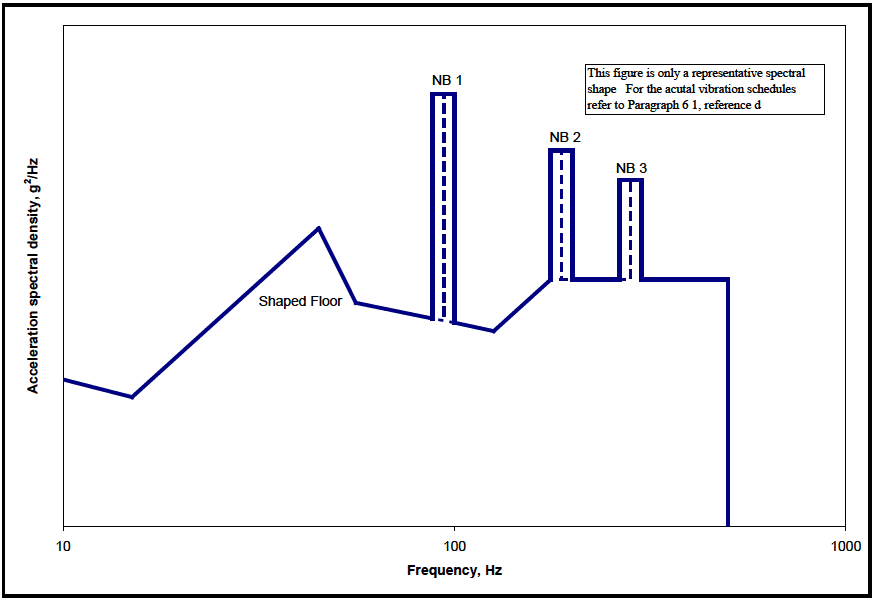
Figure description:
Acceleration Spectral Density vs. Frequency Representative spectral shape for vibration schedules
Annotations
- NB 1 (text_label - position: above peak at 100 Hz)
- NB 2 (text_label - position: above peak at ~225 Hz)
- NB 3 (text_label - position: above peak at 400 Hz)
- Shaped Floor (text_label - position: below the hump at approximately 40 Hz)
- This figure is only a representative spectral shape. For the acutal vibration schedules refer to Paragraph 6 1, reference d (text_label - position: top right corner of the chart area)
- Center frequency dashed line (vertical_line - position: x = 100)
- Center frequency dashed line (vertical_line - position: x = 225)
- Center frequency dashed line (vertical_line - position: x = 400)
| Frequency (Hz) | Acceleration spectral density (relative units) |
|---|---|
| 10 | 0.8 |
| 15 | 0.6 |
| 40 | 2.5 |
| 55 | 1.2 |
| 90 | 1.0 |
| 90 | 10.0 |
| 100 | 10.0 |
| 110 | 10.0 |
| 110 | 0.9 |
| 150 | 0.7 |
| 200 | 1.5 |
| 200 | 6.0 |
| 225 | 6.0 |
| 250 | 6.0 |
| 250 | 1.5 |
| 370 | 1.5 |
| 370 | 4.0 |
| 400 | 4.0 |
| 430 | 4.0 |
| 430 | 1.5 |
| 600 | 1.5 |
| 600 | 0.0 |
Notes: The chart displays an Acceleration Spectral Density (ASD profile on a log-log scale. The y-axis (Acceleration spectral density, g²/Hz lacks numerical values, so values in the data table are estimated relative units to capture the spectral shape. The x-axis (Frequency, Hz follows a logarithmic scale from 10 to 1000. Three narrow-band peaks, labeled NB 1, NB 2, and NB 3, are superimposed on a 'Shaped Floor'. Each narrow-band peak includes a dashed vertical line indicating its center frequency.)))
Figure 514.8D-10. Category 20 - Tracked vehicle representative spectral shape.
MIL-STD-810H METHOD 514.8, ANNEX D
2.10 Category 21 - Watercraft - marine vehicles. Note: For US Navy applications refer to Method 528.1
Marine vibration spectra have a random component induced by the variability of cruising speeds, sea states, maneuvers, etc., and a periodic component imposed by propeller shaft rotation and hull resonance. Materiel mounted on masts (such as antennas) can be expected to receive higher input than materiel mounted on the hull or deck. The overall ship's structure, materiel mounting structure, and materiel transmissibility (amplifications) greatly affect materiel vibration. Development of shipboard materiel should address both the levels of environmental inputs and the coincidence of materiel/mounting resonances and input frequencies. Gunfire shock criteria per Method 519.8 are not applicable since they are based on the response of aircraft type structures that are significantly different than marine vehicle structures.
- a. Exposure levels.
- (1) Ship/watercraft vibrations are a very complex function of natural environmental forcing function (wave action, wind), induced forcing function (propeller shaft speeds, operation of other equipment, etc.), ship/watercraft structure, materiel mounting structure and materiel response. Even roughly accurate general vibration criteria are not available. Use measurements of actual environments to develop exposure criteria.
- (2) An arbitrary qualification test requirement has been developed for shipboard materiel. This may be used as a crude definition of a total onboard life exposure. It consists of the random levels of Figure 514.8D-11 for a duration of two hours along each of three orthogonal axes, and the sinusoidal requirements of Method 528 Procedure I. In the event that actual shipboard vibration data recorded on candidate vessels show levels or frequency ranges different from those for Method 528, Procedure I, the test levels should be tailored to envelope the highest values for each frequency, with appropriate consideration given to the fatigue life of the equipment. For material to be installed in a US Navy ship any deviation from the defaults of Method 528 requires the approval of the responsible US Navy Warrant. This criterion applies to ships and not to other watercraft. No criteria are known to be available for other watercraft.
- b. Exposure durations. Take durations from the Life Cycle Environment Profile.
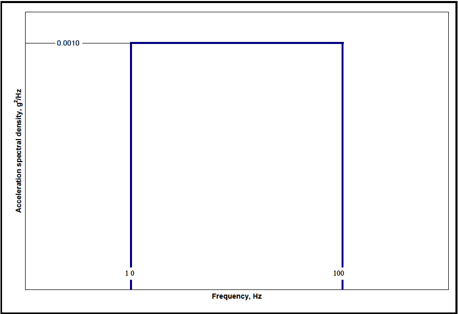
Figure description:
Power Spectral Density Profile
Acceleration spectral density vs Frequency
Annotations
- 0.0010 (text_label - position: y-axis value at 0.0010)
- 10 (text_label - position: x-axis value at 10)
- 100 (text_label - position: x-axis value at 100)
| Frequency, Hz | Acceleration spectral density, g²/Hz |
|---|---|
| 10 | 0.0000 |
| 10 | 0.0010 |
| 100 | 0.0010 |
| 100 | 0.0000 |
Notes: The graph depicts a rectangular power spectral density (PSD profile with a constant value of 0.0010 g²/Hz between the frequencies of 10 Hz and 100 Hz.)
Figure 514.8D-11. Category 21 - Shipboard random vibration exposure.
2.11 Category 22 - Engines - turbine engines
Vibration spectra for materiel mounted directly on or in close proximity to turbine engines consists of a broadband background with narrow band spikes superimposed. The broadband background is the sum of random flow turbulence and low-level quasi-sinusoidal peaks generated by various rotating machinery elements. The narrow band spikes are due to the rotation of the main engine rotor(s) and the frequencies are the rotor rotational speed(s) and harmonics.
- a. Constant speed. Many turbine engines are constant speed. This means that the rpm is held constant and power changes are made through fuel flow changes and variable pitch blades, vanes, and propellers. These machines produce the fixed frequency spikes of Figure 514.8D-12. These spikes have an associated bandwidth because there is minor rpm drift, the vibration is quasi-sinusoidal (see Annex A, paragraph 2.3.3), and the materiel resonant frequencies vary with serial number and mounting conditions.
- b. Variable speed. Other turbine engines are not constant speed machines. For these engines, the rpm varies with power setting. To represent these engines, adjust the spikes of Figure 514.8D-12 to include the engine rpm range, or alternatively, use swept sinusoidal over the engine rpm range.
- c. Multiple rotors. Multiple rotors and output shaft. Turbofan and turboshaft engines usually have two and sometimes three mechanically independent rotors operating at different speeds. Modify the spectra of Figure 514.8D-12 to include spikes for each rotor or, alternatively, used swept sinusoids for each rotor. Additionally, turboshaft engines sometimes employ gearboxes to reduce the engine output shaft speed. If the engine output shaft speed is different from one of the engine rotor speeds, modify the spectra of Figure 514.8D-12 to include spikes for the output shaft speed or, alternatively, use swept sinusoids for the output shaft speed range.
- d. Design criteria. These vibration environments can be approximated in the laboratory by the narrowband random over broadband random test described in Annex A, paragraph 2.3. Many vibration problems in this type of environment are associated with the coincidence of materiel resonant modes and the excitation spikes. The notches between spikes are used in intelligent design as safe regions for critical vibration
modes. Source dwell tests minimize the likelihood that materiel will be overstressed at non-representative conditions and that reasonable design provisions will not be subverted.
- e. Engine mounts. Engine vibration levels are affected by the engine mounting structure (see Annex A, paragraph 2.4). Thus, the same engine mounted in two different platforms may produce differing levels. Engine test stand levels are very likely to be different than platform levels. The locations of frequency peaks in the vibration spectrum are engine driven and will not change with the installation.
- f. Exposure levels. Measured values should be used when possible. For those tests employing time compression, test levels can be increased above measured values (see Annex A, paragraph 2.2) for the endurance portion of the test while measured values can be used for the performance portion of the test. Typically, component functional performance is checked at the beginning and at the end of the endurance test in each axis. Figure 514.8D-12 levels can be used when measured data are not obtainable. These levels are rough envelopes of data measured on several Air Force constant speed propeller applications.
- g. Exposure durations. Take durations from the Life Cycle Environment Profile.
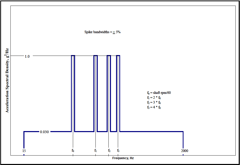
Figure description:
Acceleration Spectral Density Profile
Acceleration Spectral Density vs. Frequency Profile
Annotations
- Spike bandwidths = ± 5% (text_label - position: Upper center area above spikes)
- f₀ = shaft rpm/60 (text_label - position: Middle right area)
- f₁ = 2 * f₀ (text_label - position: Middle right area)
- f₂ = 3 * f₀ (text_label - position: Middle right area)
- f₃ = 4 * f₀ (text_label - position: Middle right area)
| Frequency (Hz) | Acceleration Spectral Density (g²/Hz) |
|---|---|
| 15 | 0 |
| 15 | 0.030 |
| 0.95 * f₀ | 0.030 |
| 0.95 * f₀ | 1.0 |
| 1.05 * f₀ | 1.0 |
| 1.05 * f₀ | 0.030 |
| 0.95 * f₁ | 0.030 |
| 0.95 * f₁ | 1.0 |
| 1.05 * f₁ | 1.0 |
| 1.05 * f₁ | 0.030 |
| 0.95 * f₂ | 0.030 |
| 0.95 * f₂ | 1.0 |
| 1.05 * f₂ | 1.0 |
| 1.05 * f₂ | 0.030 |
| 0.95 * f₃ | 0.030 |
| 0.95 * f₃ | 1.0 |
| 1.05 * f₃ | 1.0 |
| 1.05 * f₃ | 0.030 |
| 2000 | 0.030 |
| 2000 | 0 |
Notes: The chart defines a vibration spectrum with a baseline of 0.030 g²/Hz and four harmonic spikes at frequencies f₀, f₁, f₂, and f₃, each reaching 1.0 g²/Hz. The spikes have a bandwidth of ± 5% of their respective center frequencies.
Figure 514.8D-12. Category 22 - Turbine engine vibration exposure.
2.12 Category 23 - Personnel - materiel carried by/on personnel
The human body has highly damped, low frequency modes of vibration. Materiel carried on the body is protected from the vibration environment. Vibrations sufficient to harm materiel would be intolerable if transmitted through the body. Develop personnel materiel to withstand typical vibration environments (shipping, transportation, etc.) when the materiel is not carried by personnel.
- a. Exposure levels. No personal materiel vibration exposures are required.
- b. Exposure durations. No personal materiel vibration exposure durations are required.
Downloaded from https://www.everyspec.com
MIL-STD-810H METHOD 514.8, ANNEX D
(This page is intentionally blank.)
MIL-STD-810H
METHOD 514.8, ANNEX E METHOD 514.8, ANNEX E Supplemental Tailoring Guidance for Vibration Exposure Definition
NOTE: Unless specifically noted, all document references refer to paragraph 6.1 in the front part of this Method.