The following information is required to conduct and document vibration tests adequately. Tailor the lists to the specific circumstances, adding or deleting items as necessary. Although generally not required in the past, perform fixture and materiel modal surveys when practical. These data are useful in evaluating test results, and in evaluating the suitability of materiel against changing requirements or for new applications. These data can be particularly valuable in future programs where the major emphasis will be to use existing materiel in new applications. (When
modal survey is ruled out for programmatic reasons, a simple resonance search can sometimes provide useful information.)
514.8-3 DEFINITIONS
For clarity of discussion, the following definitions are provided. The definitions are not intended to be general in nature, but rather specific to the discussions in this annex.
Laboratory Vibration Test Schedule (LVTS) – All information required to perform a vibration test on a vibration exciter. Information typically includes: a broadband spectra (or profile), sine or narrowband information (if used), test run time, control accelerometer locations, control methods and tolerances, and any test specific information required.
Event – A unique exposure condition that represents some portion of the full lifecycle of a given item. Examples include flight maneuvers (i.e., forward flight at 80 percent VH) or ground vehicle conditions (i.e., paved road at 30 mph). Many events may be required to fully characterize the vibration exposure of an item.
Group – A set of events with similar vibration characteristics that are grouped together for processing.
Scenario – A tabulation of expected exposure events and the corresponding durations.
Profile – A broadband spectra that a vibration system can use as a control reference. The profile is typically provided in Auto Spectral Density (ASD) format and defined by a series of frequency and amplitude breakpoints.
Power Spectral Density (PSD) – The PSD describes how the power of a signal is distributed with respect to frequency. Vibration control systems typically use PSDs as the control reference; therefore, vibration profiles are generally developed in a PSD format. The PSD is also referred to as the auto spectral density (ASD). See Annex F, Appendix B for a description of ASD/PSD calculation methods often used. For consistency the term ASD will be used for the remainder of this Annex.
Windowing – Multiplication of a time history by a function which is zero valued outside of a given interval. Windowing is necessary for proper ASD calculation, with the Hann or Hamming windows commonly applied.
Leakage – An undesired result of windowing in which energy at one frequency leaks into adjacent frequencies. This can affect the spectral shape of the ASD and is dependent on the frequency resolution of the ASD calculations. Although the energy leaks into adjacent frequencies, the total amount of energy is preserved and the total g-rms of the ASD is unaffected.
Breakpoint – A point on the broadband profile, defined by a frequency (Hz) and a power level (g²/Hz). Breakpoints allow the multi-point profile to be represented by a reduced set of points without overly compromising the spectral information.
Miner-Palmgren Hypothesis (Miner’s Rule) – A set of mathematical equations used to scale vibration spectra and their associated test times while maintaining fatigue equivalency. A more detailed description of the Miner- Palmgren Hypothesis can be found below in paragraph 9.2.1.
Spectral Spike – Any narrowband, high-level vibration content in a vibration spectrum. The energy associated with the narrowband may be either narrowband random or sinusoidal in nature, depending upon the nature of the forcing function of the test platform. This energy is often removed from the broadband information and processed separately during analysis.
514.8-3 VEHICLE PREPARATION FOR DATA ACQUISITION - INSTALLED EQUIPMENT
Accelerometers must be mounted on the vehicle walls, deck, and roof, as well as on brackets and shelves that are integral parts of the vehicle, as close as possible to the point(s) of attachment of the existing/planned installed equipment. The purpose is to measure the vibration environment of the vehicle at the input location(s) of the installed equipment which has the same configuration as the equipment subsequently used as a test item during laboratory testing. For instance, if a piece of equipment is mounted on a bracket in the vehicle and that bracket will not appear as part of the equipment during subsequent laboratory testing, the environment should be measured on the bracket as the input to the equipment.
If a mounting platform exists and the equipment to be installed thereon is not available, use a model of the equipment with the same mass and center of gravity. This ensures that the reaction of the installed equipment will be included in the data recorded at the input to the mounting platform.
In the situation in which the test item is instrumented and may be integrated into the control scheme as such as response control or possibly as a limit location, it is critical that any surrogate hardware employed must have strong dynamic similarity to the tactical hardware. It is recommended that a comprehensive modal test of the surrogate hardware be conducted to ensure proper dynamic response is maintained. In some instances, similarity acceptance criteria may be called out, to which the modal parameters of the surrogate hardware must comply.
The difference between the mechanical impedances of mountings for field-installed and laboratory-installed equipment should be considered, particularly for relatively massive equipment. A comparison of the field and
MIL-STD-810H METHOD 514.8, ANNEX F, APPENDIX A
laboratory frequency response functions is one method of evaluating this difference, and the use of average, extreme, or response laboratory vibration control techniques is considered a valid approach to minimizing any impedance mismatch.
514.8-3 COMMON ANALYSIS FUNCTIONS AND STATISTICAL DEFINITIONS OF VSD DATA ENSEMBLES
In preparation for a VSD effort, vibration time histories are recorded for a series of test conditions (defined as “events” in Annex F, paragraph 3) also referred to as "runs". An event is defined (for ground vehicles) as operation over a specific uniform terrain, for a specific test item configuration (load, tire pressure, etc.) at a constant speed. For an aircraft, one may have a list of events defined in terms of various modes of flight (level flight, rolling maneuvers, etc.) conducted at various airspeeds. A common form of analysis involves converting the complete time history (of a particular channel) into the compressed frequency domain format of the ASD function by dividing the time history into equal length data blocks and computing the ASD for each of the data blocks independently. When combining spectra, it is assumed that the spectra being combined represent a homogeneous set. (i.e., overall spectral levels are comparable and the spectra have the same general shape). If this is not the case, combining spectra should be avoided and another "spectra category" should be added to represent the test condition. When computing estimates of these ASD functions, it is desirable to compute the linear average (assuming the number of samples is sufficiently large ), the standard deviation and the peak, all as a function of frequency, over the length of a test run. The standard deviation represents the variation in the spectral data, as a function of frequency, at a given location on the vehicle due to randomness of the test process. Although the data are stationary, excursions about the mean occur in both the time and frequency domains.
In addition to computing the mean ASD of an individual event, the standard deviation, and peak versions of the ASD are often of interest. For ease of illustration, the following symbolic structure will be employed:
G₁(f) = ASD(instantaneous) ASD computed over a single time interval T
Note that, statistically speaking, the normalized error for the (Peak) spectrum could be very high because of the limited number of degrees of freedom available from the peak values of . This spectrum is a maxi-max auto spectral density estimate and should be used with caution (if at all). An example generation of the spectra discussed above as computed from data acquired from a typical wheeled vehicle data is shown in Figure 514.8F-B.3.
MIL-STD-810H METHOD 514.8, ANNEX F, APPENDIX B
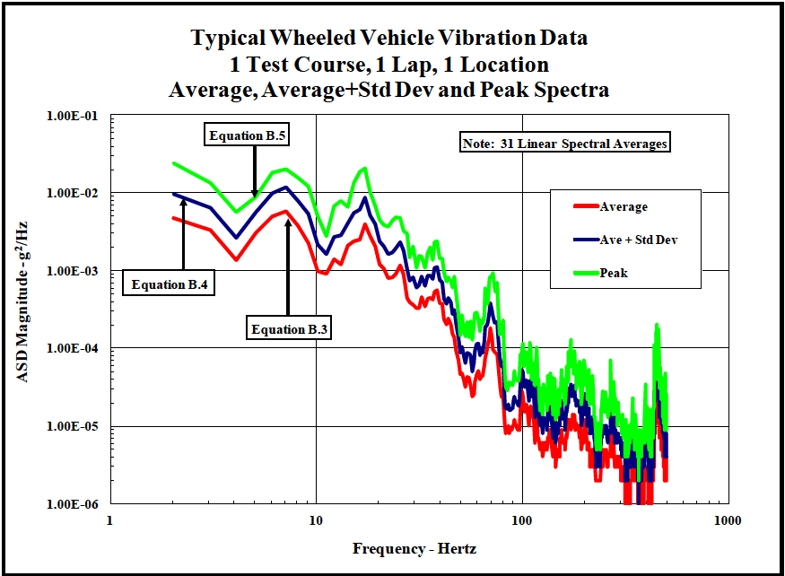
Figure description:
Typical Wheeled Vehicle Vibration Data 1 Test Course, 1 Lap, 1 Location Average, Average+Std Dev and Peak Spectra
Typical Wheeled Vehicle Vibration Data
Legend
- Average — color: red; symbol: Solid line
- Ave + Std Dev — color: dark blue; symbol: Solid line
- Peak — color: green; symbol: Solid line
Annotations
- Equation B.4 (text_label - position: Pointing to 'Ave + Std Dev' curve at approximately 2 Hz)
- Equation B.5 (text_label - position: Pointing to 'Peak' curve at approximately 5.5 Hz)
- Equation B.3 (text_label - position: Pointing to 'Average' curve peak at approximately 7.5 Hz)
| Frequency - Hertz | Average (g²/Hz) | Ave + Std Dev (g²/Hz) | Peak (g²/Hz) |
|---|---|---|---|
| 2.0 | 4.80E-03 | 9.80E-03 | 2.40E-02 |
| 3.0 | 3.40E-03 | 6.80E-03 | 1.40E-02 |
| 4.0 | 2.50E-03 | 5.20E-03 | 8.80E-03 |
| 5.0 | 1.40E-03 | 2.60E-03 | 5.60E-03 |
| 6.0 | 2.80E-03 | 5.40E-03 | 9.20E-03 |
| 7.0 | 5.40E-03 | 1.00E-02 | 1.80E-02 |
| 8.0 | 5.60E-03 | 1.10E-02 | 2.00E-02 |
| 9.0 | 4.20E-03 | 8.50E-03 | 1.60E-02 |
| 10.0 | 2.40E-03 | 4.80E-03 | 1.10E-02 |
| 11.0 | 9.50E-04 | 1.80E-03 | 3.20E-03 |
| 12.0 | 1.20E-03 | 2.20E-03 | 6.80E-03 |
| 13.0 | 1.40E-03 | 2.80E-03 | 8.10E-03 |
| 15.0 | 2.40E-03 | 5.20E-03 | 1.30E-02 |
| 17.0 | 2.60E-03 | 5.80E-03 | 1.80E-02 |
| 18.0 | 4.00E-03 | 8.80E-03 | 2.10E-02 |
| 20.0 | 2.20E-03 | 4.80E-03 | 1.20E-02 |
| 22.0 | 1.40E-03 | 3.20E-03 | 5.80E-03 |
| 25.0 | 8.20E-04 | 1.80E-03 | 4.00E-03 |
| 28.0 | 1.10E-03 | 2.20E-03 | 4.80E-03 |
| 30.0 | 6.00E-04 | 1.20E-03 | 2.60E-03 |
| 35.0 | 3.60E-04 | 7.20E-04 | 1.80E-03 |
| 40.0 | 4.00E-04 | 8.80E-04 | 1.60E-03 |
| 42.0 | 5.80E-04 | 1.20E-03 | 2.40E-03 |
| 45.0 | 3.20E-04 | 6.50E-04 | 1.10E-03 |
| 50.0 | 1.40E-04 | 3.40E-04 | 8.20E-04 |
| 60.0 | 2.80E-05 | 6.20E-05 | 2.00E-04 |
| 65.0 | 4.20E-05 | 9.20E-05 | 2.60E-04 |
| 70.0 | 5.80E-05 | 1.10E-04 | 2.40E-04 |
| 75.0 | 1.80E-04 | 3.80E-04 | 9.20E-04 |
| 85.0 | 2.40E-05 | 5.20E-05 | 1.60E-04 |
| 100.0 | 1.10E-05 | 2.20E-05 | 4.80E-05 |
| 120.0 | 5.20E-06 | 1.10E-05 | 1.10E-04 |
| 150.0 | 8.50E-06 | 1.60E-05 | 4.20E-05 |
| 200.0 | 1.40E-05 | 3.00E-05 | 1.20E-04 |
| 250.0 | 5.80E-06 | 1.40E-05 | 6.50E-05 |
| 300.0 | 3.60E-06 | 7.80E-06 | 3.40E-05 |
| 350.0 | 1.40E-06 | 3.20E-06 | 1.10E-05 |
| 400.0 | 5.40E-06 | 1.20E-05 | 3.20E-05 |
| 450.0 | 3.20E-06 | 8.20E-06 | 2.00E-04 |
| 500.0 | 2.40E-06 | 5.20E-06 | 4.80E-05 |
Notes: Note: 31 Linear Spectral Averages
Figure 514.8F-B.3. Average, average plus standard deviation, and peak spectra.
During the VSD process, classical statistics are often employed in somewhat of an ad hoc manner to address unknowns and sample size limitations. The data from many locations and many test events can be combined (by axis) using different techniques to produce representative composite spectra. The first technique is a simple linear average of all average spectra from all channels and all events to produce an overall average spectrum. If the mean and the median of the distribution are the same (which is the case for Gaussian data), this represents approximately the 50th percentile of the spectral data. A second technique is a "standard" conservative approach often integrated into the VSD process in which the ASD(Sum) spectra from each channel and each event are combined by using the average of these spectra with the addition of one standard deviation. The standard deviation computed during this process represents considerations such as the spectral variance due to location, test course differences, and courses not considered and is not the same as . Mathematically this spectral average is shown as:
Where, represents the number of events considered in the computation of the average spectra.
The standard deviation of ASD values due to variations in test courses and instrumentation locations as a function of frequency is defined as:
MIL-STD-810H
METHOD 514.8, ANNEX F, APPENDIX B
The final spectral measurement defined is: B.6
Computation of is a key component used in the VSD techniques defined in Annex F, Appendix D.
Consider the same ensemble of data as discussed in paragraph 2.7 (typical wheeled vehicle data (4 test courses, 3 data runs, 2 locations)). Figure 514.8F-B.4 includes an overlay of all 24 spectra with the average of the ensemble of spectra shown in yellow and the final representative spectrum, , shown in green.
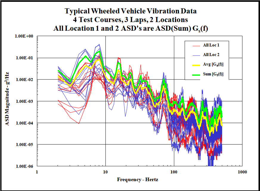
Figure description:
Typical Wheeled Vehicle Vibration Data 4 Test Courses, 3 Laps, 2 Locations; All Location 1 and 2 ASD's are ASD(Sum Gs(f
Typical Wheeled Vehicle Vibration Data
Legend
- All Loc 1 — color: red; symbol: Thin solid lines
- All Loc 2 — color: blue; symbol: Thin solid lines
- Avg [Ga(f — color: yellow; symbol: Thick solid line
- Sum [Gf(f — color: green; symbol: Thick solid line
| Frequency (Hertz) | Avg [Ga(f (g²/Hz)) | Sum [Gf(f (g²/Hz)) | All Loc 1 Range Max (g²/Hz) | All Loc 1 Range Min (g²/Hz) | All Loc 2 Range Max (g²/Hz) | All Loc 2 Range Min (g²/Hz) |
|---|---|---|---|---|---|---|
| 2 | 1.60E-02 | 2.50E-02 | 1.10E-02 | 7.00E-04 | 4.00E-02 | 3.00E-03 |
| 3 | 7.00E-03 | 1.10E-02 | 6.00E-03 | 2.00E-04 | 1.80E-02 | 2.00E-03 |
| 4 | 2.00E-02 | 3.50E-02 | 1.50E-02 | 1.00E-04 | 4.00E-02 | 3.00E-03 |
| 5 | 6.00E-02 | 1.20E-01 | 5.00E-02 | 6.00E-04 | 2.50E-01 | 1.00E-03 |
| 7 | 7.00E-02 | 1.50E-01 | 1.10E-01 | 4.00E-03 | 3.20E-01 | 5.00E-03 |
| 8 | 9.00E-02 | 2.00E-01 | 1.50E-01 | 1.00E-02 | 4.00E-01 | 8.00E-03 |
| 9 | 9.00E-02 | 2.10E-01 | 1.80E-01 | 1.50E-02 | 3.50E-01 | 7.00E-03 |
| 10 | 2.00E-02 | 4.00E-02 | 4.00E-02 | 6.00E-03 | 1.20E-01 | 4.00E-03 |
| 15 | 1.20E-02 | 2.50E-02 | 1.00E-01 | 7.00E-04 | 5.00E-02 | 4.00E-04 |
| 20 | 1.10E-02 | 1.80E-02 | 2.00E-02 | 2.00E-03 | 1.50E-02 | 3.00E-04 |
| 30 | 4.00E-03 | 7.00E-03 | 4.50E-02 | 1.50E-03 | 1.50E-02 | 6.00E-04 |
| 40 | 6.00E-03 | 1.20E-02 | 2.50E-02 | 8.00E-04 | 1.20E-02 | 1.00E-04 |
| 50 | 3.50E-03 | 6.00E-03 | 2.50E-02 | 2.00E-04 | 1.50E-02 | 6.00E-05 |
| 70 | 5.50E-03 | 1.20E-02 | 1.50E-02 | 2.00E-04 | 2.20E-02 | 3.00E-05 |
| 100 | 3.50E-04 | 7.00E-04 | 2.50E-03 | 1.50E-05 | 1.20E-03 | 8.00E-06 |
| 150 | 2.50E-04 | 5.00E-04 | 1.80E-03 | 1.00E-05 | 4.50E-03 | 5.00E-06 |
| 200 | 3.50E-04 | 7.00E-04 | 1.80E-03 | 5.00E-06 | 4.50E-03 | 4.00E-06 |
| 300 | 5.00E-05 | 1.00E-04 | 8.00E-04 | 3.00E-06 | 2.00E-03 | 2.00E-06 |
| 500 | 1.20E-04 | 3.00E-04 | 1.00E-03 | 4.00E-06 | 2.00E-03 | 2.00E-06 |
Notes: The data shows Power Spectral Density (ASD magnitudes for vehicle vibrations across a frequency range of 2 to 500 Hz on a log-log scale. Individual data series for 'All Loc 1' and 'All Loc 2' (representing 4 test courses and 3 laps each are summarized as envelope ranges in the table. The aggregate 'Avg' and 'Sum' lines are also explicitly provided.))
Figure 514.8F-B.4. Combination of 24 individual spectra.
It is desirable for a vibration schedule to be a conservative estimate of the true environment within some credible bounds. A conservative estimate is required for two reasons. First, the test sample size is limited (usually one vehicle) and some allowance must be made for differences within a class of vehicle. Second, vibration control systems take the test specification in ASD form and create a time history (to drive the shaker) by assuming a Gaussian distribution of amplitudes in the time domain. Wheeled vehicle vibration data is nearly Gaussian, but generally has larger "tails" (i.e., more data at high levels and higher peak levels) than a Gaussian distribution of the same mean and standard deviation. Since damage occurs at the tails of the distribution (and not around the mean), it is necessary to amplify the overall level so that the Gaussian process will produce the higher levels commensurate with the measured data. Merely enveloping the peak spectra provides conservatism but results in an over-test since the test rms level is generally much greater than the highest individual level measured. To ensure that the final spectral estimate is at least as large as the actual measured data, this spectrum can be adjusted (amplified or attenuated) so that its rms value is in reasonable agreement with the largest rms value measured at any location during any data run provided the corresponding spectra are similar in shape.
MIL-STD-810H METHOD 514.8. ANNEX F. APPENDIX B
The resultant spectrum shown in Figure 514.8F-B.5 is compared to an envelope of all the average spectra from the data set (in this case, 24 spectra). Note that the resultant test spectrum is approximately an envelope of the individual spectra.
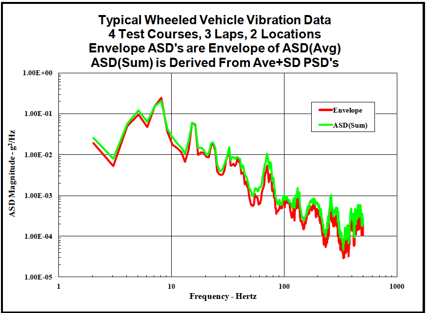
Figure description:
Typical Wheeled Vehicle Vibration Data 4 Test Courses, 3 Laps, 2 Locations; Envelope ASD's are Envelope of ASD(Avg; ASD(Sum is Derived From Ave+SD PSD's
Typical Wheeled Vehicle Vibration Data
Legend
- Envelope — color: red; symbol: thick solid line
- ASD(Sum — color: green; symbol: thick solid line
| Frequency - Hertz | Envelope (g²/Hz) | ASD(Sum (g²/Hz)) |
|---|---|---|
| 2.0 | 2.00E-02 | 2.60E-02 |
| 3.0 | 5.20E-03 | 8.00E-03 |
| 4.0 | 5.50E-02 | 5.80E-02 |
| 5.0 | 9.00E-02 | 1.20E-01 |
| 6.0 | 4.80E-02 | 6.20E-02 |
| 8.0 | 2.50E-01 | 2.20E-01 |
| 10.0 | 3.00E-02 | 4.00E-02 |
| 14.0 | 6.50E-03 | 1.20E-02 |
| 16.5 | 5.80E-02 | 6.00E-02 |
| 20.0 | 1.10E-02 | 1.50E-02 |
| 23.0 | 9.00E-03 | 1.10E-02 |
| 30.0 | 1.80E-02 | 2.00E-02 |
| 35.0 | 3.50E-03 | 4.50E-03 |
| 42.0 | 1.20E-02 | 1.60E-02 |
| 55.0 | 6.00E-04 | 1.40E-03 |
| 72.0 | 5.00E-03 | 1.10E-02 |
| 85.0 | 8.00E-04 | 1.00E-03 |
| 100.0 | 4.00E-04 | 9.00E-04 |
| 135.0 | 2.50E-04 | 1.50E-03 |
| 170.0 | 6.00E-04 | 1.00E-03 |
| 220.0 | 6.00E-05 | 1.20E-04 |
| 280.0 | 4.00E-04 | 1.00E-03 |
| 380.0 | 6.00E-05 | 4.00E-04 |
| 500.0 | 1.80E-04 | 2.50E-04 |
Notes: ASD(Sum is derived from Ave+SD PSDs. Envelope ASDs are Envelope of ASD(Avg. Data is based on 4 test courses, 3 laps, and 2 locations.))
Figure 514.8F-B.5. Comparison of resultant test spectrum (green line) to envelope of individual spectra (red line).
It is important to note that the spectrum described above may be composed of different operating conditions which are not present for the duration assigned to the total environment. For example, if certain frequency components were contributed by operation over a particular test course, they would be applied to the test as if those components occurred for the entire duration, not just the segment represented by operation over that particular test course. In this case, test duration would also apply conservatism to the process, which may or may not be desirable. Problems of this nature are addressed further in the Annex F, Appendix D.
MIL-STD-810H METHOD 514.8, ANNEX F, APPENDIX C METHOD 514.8, ANNEX F, APPENDIX C Combination of Spectra (Fatigue Damage Spectra)
514.8-3 NARROWBAND RANDOM SPECIFICATION DEVELOPMENT PROCEDURE
To allow greater flexibility in adapting to project specific requirements, the narrowband or sine tones removed from the broadband (see paragraph 2.5) can be processed in a spreadsheet. A sample narrowband random spreadsheet is provided in Table 514.8F-D.VII. The sample is of a wheeled vehicle on the 2-inch Washboard Course. Three tones were removed from each of three events (5, 7.5 and 10 mph). Note that sinusoidal processing, rather than narrowband random, would generally be used for a wheeled vehicle on the 2-Inch Washboard Course. The example is used for ease of discussion only, and will not affect the description of the process.
The following definitions provide a column-by-column description of the narrowband random processing procedures.
514.8-3 SWEPT SINE EXCITATION
The MRS is extrapolated from the MRS of fixed sinusoidal signals at frequencies corresponding to the limits of the domain of sweeping.
Example: MRS for a swept sine from 300 Hz to 1200 Hz (Figure 514.8F-E.2).
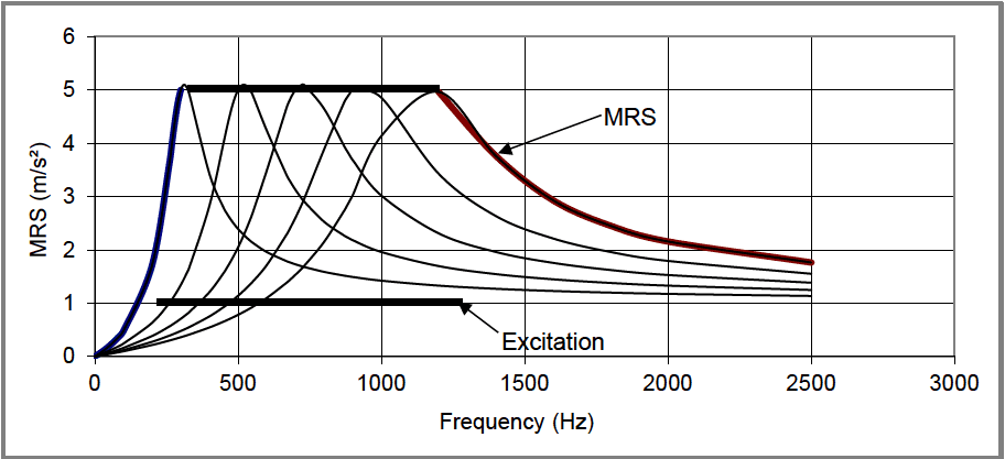
Figure description:
System Resonance Response Spectrum
MRS vs. Frequency
Legend
- MRS Envelope (Left — color: Blue; symbol: Thick solid line
- MRS Envelope (Top — color: Black; symbol: Thick solid line
- MRS Envelope (Right — color: Dark Red/Brown; symbol: Thick solid line
- Excitation — color: Black; symbol: Thick horizontal line
- Resonance Curves — color: Black; symbol: Thin solid line
Annotations
- MRS (text_label - position: Pointing to the envelope of resonance peaks and trailing slopes)
- Excitation (text_label - position: y = 1.0, x from 200 to 1250 Hz)
| Frequency (Hz) | MRS Envelope (m/s²) | Excitation (m/s²) | Curve 1 (300Hz peak) | Curve 2 (500Hz peak) | Curve 3 (700Hz peak) | Curve 4 (900Hz peak) | Curve 5 (1200Hz peak) |
|---|---|---|---|---|---|---|---|
| 0 | 0.00 | null | 0.00 | 0.00 | 0.00 | 0.00 | 0.00 |
| 100 | 0.70 | null | 0.70 | 0.40 | 0.30 | 0.20 | 0.10 |
| 200 | 2.30 | 1.00 | 2.30 | 1.20 | 0.80 | 0.60 | 0.40 |
| 300 | 5.05 | 1.00 | 5.05 | 2.20 | 1.30 | 0.90 | 0.60 |
| 400 | 5.05 | 1.00 | 2.30 | 3.50 | 1.80 | 1.20 | 0.80 |
| 500 | 5.05 | 1.00 | 1.50 | 5.05 | 2.80 | 1.70 | 1.10 |
| 600 | 5.05 | 1.00 | 1.20 | 2.80 | 4.00 | 2.20 | 1.40 |
| 700 | 5.05 | 1.00 | 1.00 | 1.80 | 5.05 | 3.20 | 1.80 |
| 800 | 5.05 | 1.00 | 0.80 | 1.50 | 3.20 | 4.20 | 2.20 |
| 900 | 5.05 | 1.00 | 0.70 | 1.30 | 2.20 | 5.05 | 2.80 |
| 1000 | 5.05 | 1.00 | 0.60 | 1.10 | 1.70 | 3.50 | 3.60 |
| 1200 | 5.05 | 1.00 | 0.50 | 0.90 | 1.30 | 2.10 | 5.05 |
| 1250 | 5.05 | 1.00 | null | null | null | null | null |
| 1400 | 3.80 | null | 0.40 | 0.70 | 1.00 | 1.50 | 3.80 |
| 1600 | 3.00 | null | 0.35 | 0.60 | 0.80 | 1.20 | 3.00 |
| 1800 | 2.50 | null | 0.30 | 0.50 | 0.70 | 1.00 | 2.50 |
| 2000 | 2.10 | null | 0.25 | 0.45 | 0.60 | 0.80 | 2.10 |
| 2500 | 1.80 | null | 0.20 | 0.35 | 0.50 | 0.70 | 1.80 |
Notes: The chart shows the Maximized Response Spectrum (MRS envelope derived from multiple resonance curves across a frequency range. The excitation level is shown as a constant floor between 200 Hz and 1250 Hz.)
Figure 514.8F-E.2. MRS for a swept sine from 300 Hz to 1200 Hz.
3.1 Pretest
The following information is required to conduct vibration tests adequately.
- a. General. See Part One, paragraphs, 5.7 and 5.9, and Part One, Annex A, Task 405 of this Standard.
- b. Specific to this Method (applicable to Procedures I through IV).
- (1) Test schedule(s) and duration of exposure(s).
- (2) Locations and specifications for all control and/or response transducers.
- (3) Test equipment limitations. Assure that test requirements (force, acceleration, velocity, displacement) can be met. Seek approval for variation if required. Document any variation.
- (4) Test shutdown procedures for test equipment or test item problems, failures, etc. (See paragraph 4.3).
- (5) Test interruption recovery procedure. (See paragraph 4.3).
- (6) Test completion criteria.
- (7) Allowable adjustments to test item & fixture (if any); these must be documented in test plan and the test report.
- c. Tailoring, Necessary variations in the basic test parameters/testing materials to accommodate LCEP requirements and/or facility limitations.
- d. Specific to Procedure.
- (1) Procedure I and IV- General and captive carriage/free flight vibration.
- i. Test fixture requirements.
- ii. Test fixture modal survey requirements / procedure.
- iii. Test item / fixture modal survey requirements / procedure.
- iv. Vibration exciter control strategy.
- v. Test tolerances.
- vi. Test temperature conditioning requirements.
- vii. Combined environment requirements (e.g., temperature, humidity).
- viii. Axes of exposure.
- (2) Procedure II - Loose cargo vibration.
- i. Orientation of test item(s) in relation to the axis of throw of the test table
- ii. Number of possible test item orientations.
- iii. Test time per orientation.
- iv. Test item temperature conditioning requirements.
- v. Test fixture requirements.
- (3) Procedure III - Large assembly transport.
- i. Test vehicle(s).
- ii. Vehicle load configuration(s).
- iii. Required road surface(s).
- iv. Required distance(s) on each road surface.
- v. Required speed(s) on each road surface.
- vi. Vehicle suspension configuration(s) i.e., tire pressures (or Central Tire Inflation System
MIL-STD-810H
METHOD 514.8
(CTIS) settings), suspension settings (as applicable) etc.
NOTE: Modal surveys of both test fixtures and test items can be extremely valuable. Large test items on large complex fixtures are almost certain to have fixture resonances within the test range. These resonances may result in significant overtests or undertests at specific frequencies and locations within a test item. Where fixture and test item resonances couple, the result can be catastrophic. Similar problems often occur with small test items, even when the shaker/fixture system is well designed because it is very difficult and often impractical to achieve a lowest fixture resonant frequency above 2000 Hz. In cases where the fixture/item resonance coupling cannot be eliminated, consider special vibration control techniques such as acceleration or force limit control.
514.8-3.1
Event (Col. A) – This column lists the events and tones (or harmonics) removed from the broadband.
3.2 During Test
Document the following information during conduct of the test:
- a. Collect the information listed in Part One, paragraph 5.10, and in Part One, Annex A, Tasks 405 and 406 of this Standard. Document any adjustments to the test item and fixture identified by the test plan, including planned stopping points. (See also paragraph 4.3.)
- b. Document the vibration exciter control strategy used, e.g., single point response, multipoint response, force limit, waveform, etc.
- c. Refer to the test-specific plan to address any additional data that may be required during the test phase.
514.8-3.2
Speed on 2” WB (Col. B) – This column contains the ground speed of the given event.
3.3 Post-Test
The following post test data, if applicable, shall be included in the test report.
- a. General. See Part One, paragraph 5.13, and Part One, Annex A, Task 406 of this Standard.
- b. Specific to this Method.
- (1) Summary and chronology of test events, test interruptions, and test failures.
- (2) Discussion and interpretation of test events.
- (3) Functional verification data.
- (4) Test item modal analysis data.
- (5) All vibration measurement data.
- (6) Documentation of any test requirement variation (paragraph 3.1 b (7))
- (7) Any changes from the original test plan.
- (8) Record of combined environment parameters (i.e., temperature and humidity).
514.8-3.3
Center Frequency Selected (Col C.) – The center frequencies of the narrowbands of interest may be set to the center frequencies of the narrowbands removed during spectral spike removal. However, it might be desirable to calculate the center frequency. For example, the center frequencies of a wheeled vehicle on a periodic course may be affected by slight changes in vehicle speed or the frequency resolution of ASD calculations. For proper control on an exciter table the tones must be harmonically related and are best set to the frequencies that would have resulted given ideal conditions. For a wheeled vehicle the frequencies can be calculated using the vehicle speed and the displacement of the periodic input (i.e., washboards spaced 0.6 meters apart). For a helicopter the frequencies can be set to the known blade passing frequency. Care should be taken to assure that the center frequency calculated does not vary significantly from the actual center frequency measured.
3.4
Test Time from Adjusted Beta Distribution (Col. D) – Generally, this column contains the times as calculated during scenario development (see Annex F, paragraph 7.1). However, the field is labeled “Adjusted” because it is sometimes necessary to combine the narrowbands of multiple events. For example, with a rotary wing aircraft the tones for all events are generally at the same frequencies (driven by the main rotor). A similar case results for narrowbands associated with tracked vehicles driven over multiple terrain types at the same speed. During processing, all narrowbands of like frequency must be combined into a single narrowband containing the combined energy of the group. Equation 9.1 or Equation 9.5 can be used to adjust the scenario times such that the g-rms of the individual narrowbands are normalized to some common g-rms, typically the maximum g-rms of the group. The adjusted test times of the individual tones (now all at the same g-rms level) are then totaled. This time is then entered into Column D of the narrowband table.
3.5
Actual Test Time (Col. E.) – This is the portion of the runtime for which the given narrowband will be within the given frequency region. Depending on the nature of the source vibration, the narrowbands will either dwell at a single frequency (i.e., helicopter) or sweep over a range of frequencies (i.e., tracked vehicle). In the case of sweeping narrowbands, the total run time selected by the analyst must be distributed across the sweep bandwidth, or the multiple narrowband breakpoints. The time is generally distributed equally between the multiple test points, with the two end points set to one half the time of the other points. See Annex F, paragraph 7.1 for an explanation of why the endpoints are treated differently.
3.6
Narrowband Bandwidth Selected (Col. F) – This field provides the width of each narrowband for vibration control. Note that the bandwidths of harmonically related tones must also be harmonically related. The bandwidth can established through a study of the individual events using pre-processing software.
3.7
Total g-rms of Tone ASD(Sum) (Col. G) – This field contains the g-rms of the narrowband energy removed from the ASD(Sum). In the case where multiple narrowbands must be combined, as discussed in paragraph 3.4, this number is the normalized g-rms used to combine the group.
3.8
Bandwidth Normalized g-rms (ASD) (Col. H.) – Modern control systems generally control to a ASD spectrum. Therefore, the g-rms values of the tones must be converted into ASD format. This is done by squaring the g-rms of Column G and dividing by the bandwidth of Column F, resulting in the g²/Hz level of Column H. This g²/Hz level represents the test level, before conservatism, associated with the test times of Column D.
MIL-STD-810H METHOD 514.8, ANNEX F, APPENDIX D Table 514.8F-D.VII. Narrowband Random Calculations
| Tone Information | Narrowband Calculations | ||||||||||
|---|---|---|---|---|---|---|---|---|---|---|---|
| Event | Speed on 2” WB | Center Freq Selected | Test Time from Adj Beta Dist | Actual Test Time | Narrowband Bandwidth Selected | Total g- rms of Tone ASD(Sum) | BandWidth Normalized g-rms (ASD) | ASD Adjusted to Test Time | Random Test Level | Ratio Adjusted to Normalized | Ratio Check |
| TONE 1 INFO | |||||||||||
| 5 mph 2” WB | 5 | 3.67 | 55.41 | 30 | 2.5 | 2.67E-01 | 2.84E-02 | 3.35E-02 | 4.69E-02 | 1.18 | |
| 7.5 mph 2” WB | 7.5 | 5.50 | 141.88 | 60 | 2.5 | 2.92E-01 | 3.42E-02 | 4.30E-02 | 6.02E-02 | 1.26 | |
| 10 mph 2” WB | 10 | 7.33 | 49.80 | 30 | 2.5 | 4.77E-01 | 9.12E-02 | 1.04E-01 | 1.46E-01 | 1.14 | |
| TONE 2 INFO | |||||||||||
| 5 mph 2” WB | 5 | 7.33 | 55.41 | 30 | 5 | 1.13E-01 | 2.57E-03 | 3.03E-03 | 4.24E-03 | 1.18 | |
| 7.5 mph 2” WB | 7.5 | 11.00 | 141.88 | 60 | 5 | 3.45E-01 | 2.38E-02 | 3.00E-02 | 4.20E-02 | 1.26 | |
| 10 mph 2” WB | 10 | 14.67 | 49.80 | 30 | 5 | 3.72E-01 | 2.77E-02 | 3.18E-02 | 4.45E-02 | 1.14 | |
| TONE 3 INFO | |||||||||||
| 5 mph 2” WB | 5 | 11.00 | 55.41 | 30 | 7.5 | 2.67E-01 | 9.50E-03 | 1.12E-02 | 1.57E-02 | 1.18 | |
| 7.5 mph 2” WB | 7.5 | 16.50 | 141.88 | 60 | 7.5 | 1.69E-01 | 3.80E-03 | 4.78E-03 | 6.69E-03 | 1.26 | |
| 10 mph 2” WB | 10 | 22.00 | 49.80 | 30 | 7.5 | 2.41E-01 | 7.77E-03 | 8.89E-03 | 1.25E-02 | 1.14 | |
MIL-STD-810H
3.13 Tracked Vehicle Considerations
The division into multiple LVTS discussed in the previous paragraph may be particularly helpful in the case of tracked vehicles. For tracked vehicles, the narrowband center frequency is a function of the vehicle speed. It may be possible to have a single broadband that represents all speeds, and to sweep the narrowband in a single sweep that encompasses all relevant speeds. However, if the broadband level changes significantly as a function of speed it may be desirable to split the multiple speeds into two or more LVTS, each of which include a given speed range.