Tailor the following paragraphs, as appropriate for the individual contract or program.
525.2-4 TIME TRACE PRE-PROCESSING
525.2-4 REPLICATION ERROR TOLERANCE SPECIFICATION
From the analyst point of view it is highly desirable to attempt to apply each of the expressions in paragraph 3 to assess the replication error. However, when it comes to TWR test tolerance specification only a few of these expressions can be easily interpreted after application. For example, requiring s(t) to be zero mean Gaussian with a specified standard deviation as a fraction of the peak values in r(t), for a test to be within tolerance is unrealistic. Requiring correlation between r(t) and s(t) to be a set value e.g., 0.975, is likewise not practical nor meaningful. The TWR test tolerance specifications below should be easily interpreted and reflect the descriptive convenience of the expressions in paragraph 3. Generally for post-analysis processing to determine test tolerance compliance it is highly desirable that replication error tolerance specifications be tailored to the form of the time history being replicated and formally agreed to before testing. The varied form of r(t), i.e., stationary, nonstationary, shock, Gaussian, non- Gaussian or any combination of all of these, requires replication error tolerance specification to be tailored based upon the form of r(t). such tolerance specification is complicated by the fact that almost assuredly some form of windowing and averaging will need to be applied for which random and bias processing errors are not easily determined to be nominal. It is usually unclear as to the reference for the specification and if multiple references need to be provided as a function of the form of r(t). In this case then there may be multiple replication error assessments and subsequent tolerance specifications.
For the suggested replication error test tolerances it is assumed that the measure of r(t) is a form of general amplitude “rms” level derived by computing the “average energy” of r(t) in terms of units-squared and then taking the square- root of this value. For Time Domain Moments this relates to the “root-energy-amplitude” except the rms duration of r(t) becomes the time averaging factor. For well defined transient vibration forms of r(t) or forms of r(t) for which root-mean-square duration is meaningful it is suggested that the reference of the specification be the “root-energy- amplitude”. For the tolerance specifications proposed below the reference “root-energy-amplitude” (REA) is provided by the following expression:
MIL-STD-810H METHOD 525.2 ANNEX B
where removal of the overall mean of 1(t) before computing REA is left to the form of r(t) and discretion of the analyst. This is a very general root-mean-square r(t) signal level and for multiple test tolerance specifications may be applied over segments of r(t). (Other possible reference scaling, for example, might be the reference range which is generally very sensitive to outliers.)
There are five general categories of replication error tolerance specifications proposed here:
The first category relates directly to s(t) and is referenced for convenience to the overall “root-mean-square" level of r(t) defined as REA above. Of the two specifications the root-mean-square error is the most significant.
Category I. The mean error, for which the STA is estimated for the oversample time interval factor on r(t), shall not exceed more than 1% of the rms amplitude of r(t), REA, over more than 5% (or 0.95 quantile) of the duration of r(t).
The root-mean-square error, for which the STA is estimated for the oversample time interval factor on r(t), shall not exceed more than 10% of the rms amplitude of r(t), REA, over more than 5% (or 0.95 quantile) of the time.
The second category relates to (1) stationary random portions of r(t), (2) a periodogram estimate i.e., ESD, over r(t) or (3) some combination of (1) and (2). For Fourier based processing of r(t) and c(t) an ASD, a periodogram or an ESD estimate is assumed available for r(t) and c(t). This includes stationary random vibration - Gaussian or non- Gaussian and shock specified in terms of an ESD estimate.
Category II. For portions of frequency domain the replication error related to the ASD or periodogram (ESD) shall not exceed the tolerance limits proposed for stationary random vibration when deterministic is considered the reference (see Method 514).
For the third category whereby a “Product Model” may be fit to of the form of a transient vibration then it is assumed that the analysis has defined in terms of a PM with a time domain rms estimate and an appropriately scaled normalized ASD estimate.
Category III. For the frequency domain portion of the PM, tolerance specification according to the Category II will apply. For the time domain portion of the PM tolerance specification according to Category I will apply.
The fourth category relates directly or as the form of a “shock” for which SRS estimates provide the most meaningful information.
Category IV. For shock the tolerance specification shall be in accord with that in Method 516. That is the tolerance specification shall not exceed the tolerance proposed for the SRS in Method 516 where deterministic is considered the reference against
The fifth category is very general and is based upon the FOT probability distribution as applied to the error . FOT is able to quantify the time for which the error is at or above a specified quantile level.
Category V. The 5th and 95th quantile of the FOT related to (for which no STA has been computed) shall not exceed more than of the plus and minus rms amplitude of .
MIL-STD-810H
METHOD 526.2
METHOD
4.1 Test Facility
Use a test facility, including all auxiliary equipment, capable of executing the TWR test with the control strategies and tolerances discussed in paragraph 4.2. In addition, use measurement transducers, data recording, and data reduction equipment capable of measuring, recording, analyzing and displaying data sufficient to document the test and to acquire any additional data required. In particular, decide on the means of determining if test tolerances have been met through either vendor supplied measures or digital post-processing measures as described in the Annexes. For TWR testing it is important that all measurements and monitoring of test item functioning be correlated in time.
525.2-4.1 Introduction
Not many post-test analysis procedures (independent of vendor supplied test analysis) have been formally established and agreed upon for quantifying the replication error. For one-of-a-kind type testing with a unique reference time trace, some reliance should be made upon custom software in post-test analysis to verify test tolerance satisfaction.
Figure 525.2A-2 displays the TWR control time traces for (H) and (S) configurations (along with the same reference time trace) prior to beginning of preprocessing where the time traces have been truncated for convenience.
MIL-STD-810H METHOD 525.2 ANNEX A
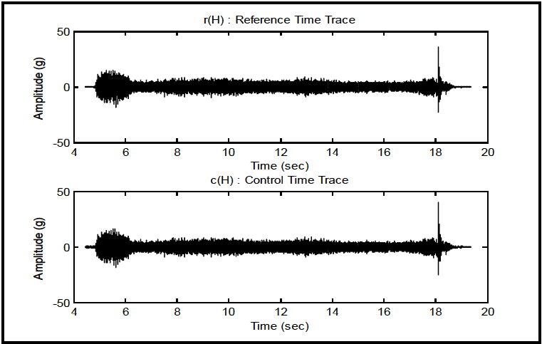
Figure description:
Reference and Control Time Traces
r(H : Reference Time Trace
Annotations
- High amplitude spike (vertical_line - position: Time = 18.1 sec)
- Initial burst (shaded_area - position: Time = 4.8 to 6.2 sec)
| Time (sec) | Min Amplitude (g) | Max Amplitude (g) |
|---|---|---|
| 4.0 | 0.0 | 0.0 |
| 4.5 | -1.0 | 1.0 |
| 4.8 | -5.0 | 5.0 |
| 5.0 | -12.0 | 12.0 |
| 5.5 | -16.0 | 16.0 |
| 6.0 | -12.0 | 12.0 |
| 6.5 | -7.0 | 7.0 |
| 7.5 | -6.0 | 6.0 |
| 8.5 | -6.0 | 6.0 |
| 9.5 | -7.0 | 7.0 |
| 10.5 | -7.0 | 7.0 |
| 11.5 | -8.0 | 8.0 |
| 12.5 | -8.0 | 8.0 |
| 13.5 | -9.0 | 10.0 |
| 14.5 | -9.0 | 10.0 |
| 15.5 | -8.0 | 8.0 |
| 16.5 | -8.0 | 8.0 |
| 17.5 | -10.0 | 10.0 |
| 18.0 | -12.0 | 12.0 |
| 18.1 | -22.0 | 36.0 |
| 18.5 | -5.0 | 5.0 |
| 19.0 | -2.0 | 2.0 |
| 19.5 | 0.0 | 0.0 |
c(H : Control Time Trace
Annotations
- High amplitude spike (vertical_line - position: Time = 18.1 sec)
- Initial burst (shaded_area - position: Time = 4.8 to 6.2 sec)
| Time (sec) | Min Amplitude (g) | Max Amplitude (g) |
|---|---|---|
| 4.0 | 0.0 | 0.0 |
| 4.5 | -1.0 | 1.0 |
| 4.8 | -5.0 | 5.0 |
| 5.0 | -12.0 | 12.0 |
| 5.5 | -16.0 | 16.0 |
| 6.0 | -12.0 | 12.0 |
| 6.5 | -7.0 | 7.0 |
| 7.5 | -6.0 | 6.0 |
| 8.5 | -6.0 | 6.0 |
| 9.5 | -7.0 | 7.0 |
| 10.5 | -7.0 | 7.0 |
| 11.5 | -8.0 | 8.0 |
| 12.5 | -8.0 | 8.0 |
| 13.5 | -9.0 | 10.0 |
| 14.5 | -9.0 | 10.0 |
| 15.5 | -8.0 | 8.0 |
| 16.5 | -8.0 | 8.0 |
| 17.5 | -10.0 | 10.0 |
| 18.0 | -12.0 | 12.0 |
| 18.1 | -22.0 | 40.0 |
| 18.5 | -5.0 | 5.0 |
| 19.0 | -2.0 | 2.0 |
| 19.5 | 0.0 | 0.0 |
Notes: Both charts show nearly identical time traces of amplitude in g over a 20-second interval, featuring an initial high-energy burst and a late sharp spike.
Figure 525.2A-2a. Exciter head (H) (reference/control time traces prior to post-test preprocessing).
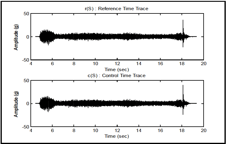
Figure description:
Reference and Control Signal Time History
r(S : Reference Time Trace
| Time (sec) | Min Amplitude (g) | Max Amplitude (g) |
|---|---|---|
| 4.0 | 0 | 0 |
| 4.5 | 0 | 0 |
| 4.8 | 0 | 0 |
| 5.0 | -12 | 12 |
| 5.2 | -15 | 15 |
| 5.5 | -18 | 18 |
| 5.8 | -15 | 15 |
| 6.0 | -10 | 10 |
| 6.3 | -5 | 5 |
| 7.0 | -8 | 8 |
| 8.0 | -10 | 10 |
| 9.0 | -10 | 10 |
| 10.0 | -10 | 10 |
| 11.0 | -10 | 10 |
| 12.0 | -12 | 12 |
| 13.0 | -10 | 10 |
| 14.0 | -10 | 10 |
| 15.0 | -10 | 10 |
| 16.0 | -10 | 10 |
| 17.0 | -10 | 10 |
| 17.5 | -10 | 10 |
| 17.8 | -12 | 12 |
| 18.0 | -15 | 15 |
| 18.1 | -25 | 38 |
| 18.2 | -10 | 10 |
| 18.4 | -5 | 5 |
| 18.6 | -2 | 2 |
| 19.0 | 0 | 0 |
| 20.0 | 0 | 0 |
c(S : Control Time Trace
| Time (sec) | Min Amplitude (g) | Max Amplitude (g) |
|---|---|---|
| 4.0 | 0 | 0 |
| 4.5 | 0 | 0 |
| 4.8 | 0 | 0 |
| 5.0 | -12 | 12 |
| 5.2 | -15 | 15 |
| 5.5 | -18 | 18 |
| 5.8 | -15 | 15 |
| 6.0 | -10 | 10 |
| 6.3 | -5 | 5 |
| 7.0 | -8 | 8 |
| 8.0 | -10 | 10 |
| 9.0 | -10 | 10 |
| 10.0 | -10 | 10 |
| 11.0 | -10 | 10 |
| 12.0 | -12 | 12 |
| 13.0 | -10 | 10 |
| 14.0 | -10 | 10 |
| 15.0 | -10 | 10 |
| 16.0 | -10 | 10 |
| 17.0 | -10 | 10 |
| 17.5 | -10 | 10 |
| 17.8 | -12 | 12 |
| 18.0 | -15 | 15 |
| 18.1 | -25 | 40 |
| 18.2 | -10 | 10 |
| 18.4 | -5 | 5 |
| 18.6 | -2 | 2 |
| 19.0 | 0 | 0 |
| 20.0 | 0 | 0 |
Notes: Both charts show the high-frequency amplitude signal over time. The control trace c(S appears to track the reference trace r(S very accurately, reproducing the initial burst at ~4.8-6.3 seconds, the steady-state vibration through ~17.8 seconds, and the sharp impulse at ~18.1 seconds.))
Figure 525.2A-2b. Exciter slip table (S) (reference/control time traces prior to post-test preprocessing).
Before the reference and control time traces are processed and the difference time trace is generated, some preprocessing is necessary. Preprocessing must be performed in both the time and frequency domains. The following preprocessing procedures will be discussed in turn:
- a. Frequency Band Limiting.
- b. Time Trace Correlation.
- c. Time Trace Segment Identification.
MIL-STD-810H METHOD
4.1.1 Procedure I - The SESA Replication of a Field Measured Materiel Time Trace Input/Response
The SESA replication of a field measured time trace representing an input to the materiel or a response of the materiel considers only an un-scaled measured time trace in the laboratory with a single exciter in a single axis or mechanical degree-of-freedom.
4.1.2 Procedure II - The SESA Replication of an Analytically Specified Materiel Time Trace Input/Response
The SESA replication of an analytically specified time trace representing an input to the materiel or a response of the materiel considers carefully scaled versions of a measured time trace in the laboratory with a single exciter in a single axis or mechanical degree-of-freedom.
4.2 Controls
525.2-4.2 Frequency Band Limiting
The objective of frequency band limiting is to ensure for time trace comparison, the reference and control time traces exist over the same exact frequency band (generally a bandwidth coincident with the TWR control bandwidth). The importance of this operation cannot be over emphasized. If the control time trace has significant high frequency information not contained in the reference time trace (as a result of boundary conditions or impedance mismatch), this will be reflected in any TPP amplitude comparisons. The band pass filter to provide a common bandwidth for the time traces is selected such that the minimum of the reference bandwidth and the control bandwidths is established. This common bandwidth may be specified as, e.g., 10 Hz to 2000 Hz, or determined by examining the magnitude of a periodogram estimate for both time traces. The frequency band limiting operation is performed on both the reference and control time traces, and always performed before time trace correlation considerations. Unless the time traces are excessive in length, a single block rectangular window FFT magnitude (periodogram) plotted in dB for both the reference and control time traces is satisfactory for identifying the common bandwidth. For excessively long time traces, the Welch method of spectrum computation may be employed for common bandwidth identification. To obtain the common bandwidth, a standard bandpass filter may be applied, making sure to preserve filter phase linearity, in obtaining the reference and control time traces. Figure 525.2A-3 provides single block periodograms for the reference and control time traces before and after bandpass filtering.
NOTE: With regard to frequency band-limiting, it is very important that for any field time trace measurement program designed to provide input to TWR laboratory testing, the bandwidth of the field measurements exceeds by definition, the bandwidth of interest for laboratory testing (TWR test control bandwidth). For example, if test specifications call for a 10 Hz to 2000 Hz laboratory test bandwidth, the field time trace measurements must exceed 2000 Hz, e.g., 4000 Hz, in order to provide a reference time trace with sufficient bandwidth to compare with the unprocessed control time trace resulting from TWR laboratory testing. Less critically field measurements would have frequency content below 10 Hz, e.g., 5 Hz. The rationale behind this is as follows. Almost certainly the laboratory test will exhibit energy out of the test specification frequency band of interest or the exciter test control bandwidth as a result of mismatch of materiel/test fixture/exciter impedance/boundary conditions. To directly compare the field reference time trace (before bandwidth limiting as a TWR input) with the unprocessed laboratory control time trace, (even though the reference time trace may have been bandlimited for laboratory test), the field measured reference time trace must have a bandwidth consistent with the unprocessed laboratory control time trace, i.e., a bandwidth that encompasses the bandwidth of the unprocessed laboratory control time trace. Thus, bandlimiting for comparison of reference and control time traces must be in accord with the most significant energy in the unprocessed laboratory control time trace (that likely exceeds the test specification bandwidth). Comparison for purposes of time trace peak modeling for the reference and control time trace is particularly sensitive to frequency bandlimiting considerations. To compare reference and control time trace information in terms of the full bandwidth that the materiel experienced in laboratory test, the laboratory test control bandwidth must determine the bandwidth for comparison. In the example provided here the field measured reference time trace was bandlimited to 2000 Hz (by measurement system design without TWR consideration) thus, by necessity, in comparison, the measured reference time trace somewhat “incorrectly” controls bandwidth for comparison. As noted, TWR testing has important implications for field measurement system design.
MIL-STD-810H
METHOD 525.2 ANNEX A
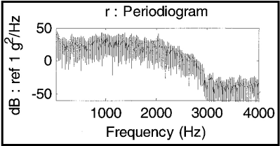
Figure description:
r : Periodiogram
r : Periodiogram
| Frequency (Hz) | Magnitude (dB : ref 1 g²/Hz) |
|---|---|
| 0 | 40 |
| 250 | 30 |
| 500 | 25 |
| 750 | 35 |
| 1000 | 30 |
| 1250 | 35 |
| 1500 | 30 |
| 1750 | 25 |
| 2000 | 30 |
| 2250 | 20 |
| 2500 | 10 |
| 2750 | -5 |
| 3000 | -40 |
| 3250 | -45 |
| 3500 | -45 |
| 3750 | -45 |
| 4000 | -40 |
Notes: The graph displays a power spectral density (PSD periodogram. The plot shows high energy in the lower frequencies up to approximately 2500 Hz, followed by a sharp roll-off between 2500 Hz and 3000 Hz, after which the signal levels out into a lower noise floor.)
(a) Reference Time Trace
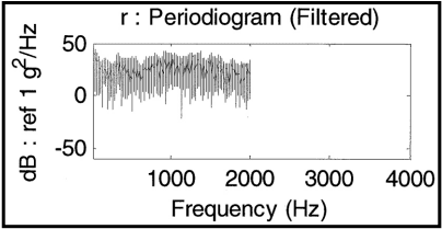
Figure description:
r : Periodiogram (Filtered
r : Periodiogram (Filtered
| Frequency (Hz) | Signal (Dark Line (dB)) | Signal Range Lower Bound (dB) | Signal Range Upper Bound (dB) |
|---|---|---|---|
| 0 | 38 | 5 | 48 |
| 100 | 30 | -5 | 40 |
| 200 | 26 | -10 | 38 |
| 300 | 22 | -15 | 35 |
| 400 | 24 | -5 | 38 |
| 500 | 20 | -10 | 36 |
| 600 | 28 | 5 | 40 |
| 700 | 24 | -2 | 38 |
| 800 | 26 | 0 | 42 |
| 900 | 32 | 10 | 45 |
| 1000 | 30 | 8 | 42 |
| 1100 | 22 | -25 | 38 |
| 1200 | 34 | 12 | 45 |
| 1300 | 28 | 5 | 41 |
| 1400 | 32 | 10 | 43 |
| 1500 | 25 | -5 | 40 |
| 1600 | 30 | 8 | 42 |
| 1700 | 22 | -10 | 38 |
| 1800 | 18 | -15 | 32 |
| 1900 | 25 | -8 | 36 |
| 2000 | 22 | -12 | 35 |
| 2100 | null | null | null |
| 3000 | null | null | null |
| 4000 | null | null | null |
Notes: The chart shows a frequency spectrum that is heavily filtered above 2000 Hz, where signal magnitude drops to negligible levels. The 'Signal Range' represents the vertical bar variations seen in the original plot.
(b) Bandlimited Reference Time Trace (10 Hz – 2000 Hz)
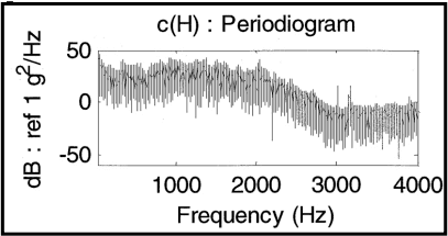
Figure description:
c(H : Periodogram
c(H : Periodogram
| Frequency (Hz) | Power Spectral Density (dB : ref 1 g²/Hz) |
|---|---|
| 0 | 42 |
| 200 | 35 |
| 400 | 32 |
| 600 | 28 |
| 800 | 40 |
| 1000 | 45 |
| 1200 | 40 |
| 1400 | 35 |
| 1600 | 38 |
| 1800 | 32 |
| 2000 | 38 |
| 2200 | 20 |
| 2400 | 15 |
| 2600 | 5 |
| 2800 | -10 |
| 3000 | 15 |
| 3200 | 12 |
| 3400 | -15 |
| 3600 | -18 |
| 3800 | -10 |
| 4000 | 0 |
Notes: The periodogram displays a high-frequency oscillatory signal with a dense set of spectral components. The values in the table represent the approximate peak envelope and significant discrete spectral spikes (notably near 3000 Hz and 3200 Hz. The overall trend shows a decrease in power density as frequency increases from 2000 Hz towards 3500 Hz.)
(c) Control Time Trace Exciter Head (H)
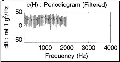
Figure description:
c(H : Periodogram (Filtered
c(H : Periodogram (Filtered
| Frequency (Hz) | Magnitude Trend (dB : ref 1 g²/Hz) | Magnitude Upper Bound (dB : ref 1 g²/Hz) | Magnitude Lower Bound (dB : ref 1 g²/Hz) |
|---|---|---|---|
| 0 | 40 | 48 | 10 |
| 200 | 32 | 42 | 2 |
| 400 | 28 | 38 | 5 |
| 600 | 25 | 40 | -8 |
| 800 | 30 | 44 | 0 |
| 1000 | 32 | 45 | 5 |
| 1200 | 28 | 42 | -10 |
| 1400 | 30 | 44 | -5 |
| 1600 | 26 | 38 | -8 |
| 1800 | 22 | 35 | -12 |
| 2000 | 24 | 36 | -15 |
Notes: The data plotted ends at 2000 Hz, while the x-axis scale extends to 4000 Hz. The periodogram exhibits high frequency noise, represented here by trend, upper, and lower bounds.
(d) Bandlimited Control Time Trace Exciter Head (H) (10 Hz – 2000 Hz)
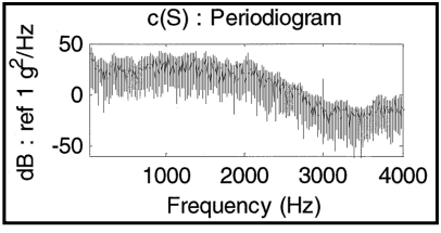
Figure description:
c(S : Periodogram
c(S : Periodogram
Legend
- Smoothed Level — color: black; symbol: Solid line
- Periodogram — color: gray; symbol: Vertical lines
| Frequency (Hz) | Smoothed Level (dB) | Periodogram Min (dB) | Periodogram Max (dB) |
|---|---|---|---|
| 0 | 35 | 10 | 50 |
| 250 | 25 | -5 | 40 |
| 500 | 25 | -15 | 40 |
| 750 | 25 | -5 | 40 |
| 1000 | 30 | 0 | 45 |
| 1250 | 35 | 5 | 45 |
| 1500 | 30 | 0 | 45 |
| 1750 | 25 | -5 | 45 |
| 2000 | 25 | -20 | 45 |
| 2250 | 20 | -25 | 40 |
| 2500 | 10 | -30 | 25 |
| 2750 | 0 | -40 | 15 |
| 3000 | -10 | -50 | 15 |
| 3250 | -20 | -55 | -10 |
| 3500 | -25 | -60 | -15 |
| 3750 | -15 | -50 | 0 |
| 4000 | -15 | -45 | 0 |
Notes: The chart displays a periodogram of a signal c(S. The gray vertical bars show the raw periodogram data, while the solid black line represents a smoothed spectral estimate. A notable narrow spike is present at approximately 3000 Hz.)
(e) Control Time Trace Slip Table (S)
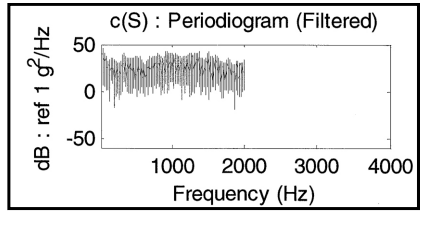
Figure description:
c(S : Periodogram (Filtered
c(S : Periodogram (Filtered
| Frequency (Hz) | Upper Bound Magnitude (dB) | Lower Bound Magnitude (dB) | Estimated Mean (dB) |
|---|---|---|---|
| 0 | 48 | 35 | 42 |
| 200 | 38 | -15 | 25 |
| 400 | 42 | 5 | 28 |
| 600 | 38 | -5 | 25 |
| 800 | 42 | 5 | 30 |
| 1000 | 46 | -5 | 35 |
| 1200 | 44 | 5 | 30 |
| 1400 | 45 | -10 | 28 |
| 1600 | 41 | 0 | 26 |
| 1800 | 36 | -5 | 24 |
| 2000 | 35 | -20 | 20 |
Notes: The data series stops at approximately 2000 Hz, although the x-axis continues to 4000 Hz. The plot represents a filtered periodogram with high variance, shown as vertical spikes around a central trend line. The y-axis unit is dB relative to 1 g²/Hz.
(f) Bandlimited Control Time Trace Slip Table (S) (10 Hz – 2000 Hz)
Figure 525.2A-3. Reference/control time trace periodograms for frequency band limiting through FFT window filtering.
Based upon examination of the periodograms for both time traces in Figure 525.2A-2, the very low frequency information (below 10 Hz), and the very high frequency information (above 2000 Hz) is filtered out. The frequency analysis bandwidth for this operation is 0.067 Hz.
4.3 Time Trace Correlation.
After a common frequency bandwidth has been established, it is essential that the band limited reference and control time traces be “perfectly” or “maximally” correlated in time (i.e., one time trace is not shifted in time relative to the other time trace) for TPP assessment. If the vendor software does not guarantee this perfect correlation in time, the degree of correlation must be checked. To perform this check and take corrective action, the cross-covariance function estimate is determined, and the time traces shifted relative to one another, such that the peak in the cross-covariance function estimate appears at the zero cross-covariance lag. This computation should be performed, if possible, on a reasonably stationary segment of the time trace. It is unnecessary to perform the correlation computations over the entire trace, but only necessary to get a long-enough segment such that the degree of shift can be determined with
MIL-STD-810H METHOD
4.2.1 Calibration
Ensure for the exciter system, all transducers, signal conditioning equipment, independent measurement systems, and the exciter control system hardware are calibrated for conformance with the specified test requirement(s). Ready access to the reference, control, and drive time trace files in ASCII form will be required for independent confirmation of adequacy of the time trace replication for a successful TWR test.
4.2.2 Tolerances
- a. General Philosophical Discussion. At this point in TWR test methodology, test tolerance specification is not well quantified. Test tolerance development for TWR is based upon a different laboratory test philosophy as opposed to the test philosophy contained in Methods 514.8 and 516.8. The reason for this change in philosophy is embedded in the implementation of TWR testing. TWR testing may involve replicating a combination of stationary Gaussian, stationary non-Gaussian, and nonstationary measured environments within a single time trace designated the reference time trace. Tolerance specification may be related to current tolerance specification in Methods 514.8 and 516.8, or be independently established based upon the nature of TWR testing. First, it is important to note that TWR does not provide a “waveform control strategy” that implies the satisfaction for the time control trace of each of the time/amplitude coordinates of every point within the reference time trace (satisfaction to within some predetermined amplitude tolerance, while totally satisfying the sampling time constraint). Exciter control and feedback hardware/software configurations to accomplish this to a bandwidth of 2000 Hz are currently not available. TWR implicitly “averages” the reference time trace (waveform) information over both time and frequency. There are two sources for the time and frequency averaging. The first source is through compensation of the voltage drive waveform by linear convolution of the exciter system impulse response function estimate with the reference time trace. The condition of system linearity is almost never satisfied so that the reference time trace is averaged over time through the linear convolution (as opposed to providing convolution through a two-dimensional non-stationary/nonlinear impulse response function that changes instantaneously in time). The second source is the implicit and nearly unavoidable averaging of significant amounts of energy from signals outside of the reference time trace bandwidth (i.e., the bandwidth for TWR control). These two sources of time/frequency averaging severely limit consideration of time point (or increment) by time point (or increment) amplitude tolerance limit specification between the reference and control time traces. Experience has shown that the distribution of the time point by time point difference between the reference and control
time traces is almost always non-Gaussian distributed, leading to the need for a complex tolerance specification and interpretation. Even though this may seem to be a significant limitation for the implementation of TWR testing, it is important to realize that the focus of TWR is replication of a stochastic field environment for which any one measured sample time trace (out of a potentially infinite number of such traces) has a zero probability of occurrence. Because the exact probability structure of the "true" field environment is generally unknown, this implies that the test tolerance specification can be quite broad, and the objective of the test (be it structural integrity or functional capability) can be satisfied at the same time. In the broadest interpretation, this can border on concluding that if the reference and control time traces plotted side-by-side visually "look alike", then tolerance in terms of random process theory and sample functions has been met, even though the time-point by time-point amplitude (TPP) difference between the reference and control traces may be substantial. In the tolerance consideration for this Method, although TPP provides an interesting display by plotting the reference time trace versus the control time trace along orthogonal axes (see Annex A), it is not recommended that TPP comparison be the major determiner for test tolerance satisfaction. Instead, recommend that time and frequency average estimates made over the same time frame on the reference and control time traces be used for tolerance specification. In particular, it is recommended that frequency based averages incorporated into ASD, SRS estimation, and time-based averages incorporated into mean-square (or root-mean-square) estimation be used in tolerance specifications whenever possible. Methods 514.8 and 516.8 incorporate test tolerances on ASD and SRS estimates, respectively. The tolerances in these two methods are easily interpreted, and generally are easily satisfied in TWR testing. With regards to time based averages, it is important to note that while the root-mean-square of the difference between two independently distributed Gaussian random variables is a function of the square-root of the sum of their variances, the difference of the root-mean-square levels of the two random variables (averaged over a certain number of realizations) may be an order of magnitude or more less. That is, the variance of an average of variables from a probability distribution with variance is . Annexes A and B discuss the form for tolerance specification in more detail. In the paragraphs to follow, the term "Specialized Test Tolerance Requirements" (STTR) will be used. Use of STTR recognizes that TWR testing may require a level of sophistication in environmental test tailoring not experienced in the standard methods. For example, materiel exposed to high levels of kurtosis may require TWR test methodology based upon field measurements. Such a specialized laboratory test may require verification of the kurtosis levels, and a detailed specification of the shape of the probability density function to ensure other probability distribution moments are acceptable. It is not feasible in this Method to prescribe acceptable tolerance limits for this scenario. Thus, such tolerance limits will be developed under the term STTR and will require trained analysts for specification and interpretation. This allows the focus in paragraphs 4.2.2b and 4.2.2c of a more practical nature.
- b. Practical Tolerance Considerations. Laboratory testing in another method that is implemented by using TWR test methodology should be under laboratory test tolerance requirements in the other method. For example, Method 516.8 provides tolerances on shock under the SRS methodology. For a measured shock time trace replicated under TWR test methodology, the same SRS based test tolerances should apply for comparison of the reference time trace SRS with the control time trace SRS. In general, tolerances specified for TWR test methodology should be consistent with, and no broader than laboratory test tolerances in other methods for testing with similar objectives. Relative to TWR test methodology on measured time traces of diverse form, measured mechanical response time traces and portions of such time traces may have any one of three characteristic forms.
- (1) The first form is that of Gaussian or non-Gaussian stationary random vibration.
- (2) The second form is that of a short duration high level transient or shock where the duration of the transient is much shorter than the periods of the lowest natural frequencies of interest for the materiel.
- (3) The third form is that of a non-stationary transient vibration having duration that substantially exceeds the period of the lowest natural frequency of the materiel.
A fourth form, too specialized for consideration here, might be classed as periodic repetition of an event for which test tolerance is established according to time trace ensemble statistics (see Method 519.8, Gunfire Shock). For TWR tolerance development, such tolerances should not exceed the tolerances provided for
|
|
stationary random vibration and mechanical shock for the first and second forms, respectively. It is anticipated that a properly designed TWR test will easily meet the tolerance levels specified in both of these forms (Methods 514.8 and 516.8). The tolerances for the third form of non-stationary time trace are somewhat dependent upon the nature of the non-stationarity. Techniques for non-stationarity assessment in which time trace amplitude is a function of both time and frequency are available (see paragraph 6.1 references a and b). Some non-stationary time traces that have time invariant frequency characteristics can be represented by the Product Model (PM), and can be processed for tolerance purposes as stationary random vibration with a time-varying envelope. Annexes A and B should be consulted for details of TWR tolerance specification for non-stationary time traces. If it is unclear as to how to segment a TWR time trace, then (1) time-average test tolerances may be provided on the difference between the control and reference time traces, or (2) digital bandpass filtering may be performed on both the control and reference time traces to make common bandwidth comparisons. The Annexes should be consulted for such tolerance development.
- c. Tolerance Recommendations. In general, all test tolerances need to be established by some comparison in the time domain and frequency domain of the digitized reference and control time traces. Rudimentary comparison that might be taken for nominal test tolerances is usually performed by the vendor-supplied TWR software. The vendor will typically refer to the rudimentary comparison as “rms error.” Test laboratory personnel need to consult the vendor supplied TWR system manuals for such error considerations, and have a very clear understanding of the proper interpretation and meaning of such error; in particular, the segment size and averaging performed in order to establish the “rms error.” It is strongly advised that TWR test tolerances be developed independently of vendor supplied software, and verification of the satisfaction of TWR test tolerances be performed independently of vendor supplied software. In addition, in no case should vendor supplied software be relied upon for the specification of TWR test tolerances. However, it is vitally important that specified TWR test tolerances be correlated in some general manner with vendor supplied “rms error,” so that test interruption may be performed if large “rms error” implies specified test tolerance exceedance above a prescribed limit. If testing occurring in real time at levels exceeding the maximum test tolerance rms error limit by 10 percent, the test needs to be interrupted. Generally, it is essential that for a precise comparison (1) the reference and control time traces be band-limited to the exact SESA frequency band of interest, and (2) the reference and control time traces be maximally correlated by way of digital pre-processing (see Annex A). After such pre-processing, recommend the reference time trace be segmented into portions that might be considered stationary, short transient (or shock) and long transient. Generally, a 10 percent tapered cosine window should be applied to each of the segments such that the characteristic part of the time trace is scaled by unity, and the end points are zero. It is assumed that good signal processing practices are used to determine the basic estimates for deciding tolerance satisfaction (see Annex B). In particular, this may mean balancing the statistical random and bias error in the estimates. ASD and mean-square envelope estimates are susceptible to statistical processing errors that may distort the resulting estimates.
- (1) Stationary Gaussian or non-Gaussian (may include discrete components):
- (a) Frequency domain: For a cosine windowed segment represented by a Gaussian or non-Gaussian stationary random time trace, tolerances are placed upon ASD estimates. The control time trace ASD estimate is to be consistent with the tolerances given in Method 514.8.
- (b) Amplitude domain comparison (STTR): When the windowed segment of the reference time trace is non-Gaussian (incorporates skewness, kurtosis or both skewness and kurtosis), recommend the plotting of the reference and control along orthogonal axes be initially performed for visual inspection. This visual inspection should then be followed by an empirical quantile plot of reference time trace amplitudes versus control time trace amplitudes (qq plot). The qq point plot should approach a straight line at forty-five degrees to each axis. Confidence intervals on this line according to the sample size can be used for tolerance specification STTR. Histogram plots of the reference and control time traces for enhanced tail structure may provide useful visual inspection, and can be used for tolerance specification for STTR. Finally, estimates of the non-Gaussian probability distribution parameters may be compared between the reference and the control time traces, exercising caution since the parameter value estimates are subject to quite restrictive statistical error considerations. For a zero mean reference time trace, ensure single estimates of the overall time trace sample variance are within ±10 percent of the reference time trace. Probability density of reference and control signals should be compared to observe skewness and kurtosis characteristics.
MIL-STD-810H
METHOD 525.2
(2) Shock:
- (a) Frequency domain: For an appropriately windowed segment represented by a shock, ensure the tolerance on the control time trace SRS estimate with 5 percent critical damping is within -6dB and+ 3dB of the reference time trace SRS estimate for at least a one-twelfth octave bandwidth resolution.
- (b) Amplitude domain: For the segment, ensure the major (maximum absolute magnitude) positive and negative peaks (not to exceed 10 percent of all the reference time trace peaks in number) in the control time trace are within ± 20 percent magnitude of the corresponding peaks in the reference time trace (peak correspondence is based upon the fact that the control and reference time traces have zero phase shift between them).
- (3) Nonstationary (Product Model):
- (a) Amplitude domain: For an appropriately windowed segment that can be represented by the “Product Model,” suggest the short-time average estimate of the control time trace envelope (time average root-mean-square level) be within ±1 dB of the short-time average estimate of the reference time trace envelope, where the short-time averaging time (and time shift in average time estimates) is not to exceed 1 percent of the total duration of the reference time trace.
- (b) Frequency domain comparison: Ensure the normalized ASD estimate for the control time trace is within ±3.0 dB (ratio of approximately 2) of the normalized ASD estimate for the reference time trace over a significant portion of the bandwidth. Note: this may seem a broad tolerance bound but generally the normalized ASD estimates have a restricted number of statistical degrees-of-freedom.
Annex A illustrates processing for test tolerance satisfaction. Annex B provides a table of analytical formulas and some preliminary test tolerance specifications that may be used to formally specify tailored test tolerance (in particular, for STTR). In cases where specified tolerances cannot be met, achievable tolerances should be established and agreed to by the cognizant engineering authority and the customer prior to initiation of the test.
Test interruptions can result from multiple situations. The following paragraphs discuss common causes for test interruptions, and recommended paths forward for each. Recommend test recording equipment remain active during any test interruption if the excitation equipment is in a powered state.
4.3 Test Interruption
Test interruptions can result from a number of situations that are described in the following paragraphs.
4.3.1 Interruption Due To Laboratory Equipment Malfunction
- a. General. See Part One, paragraph 5.11, of this Standard.
- b. Specific to this Method. When interruptions are due to failure of the laboratory equipment, analyze the failure to determine root cause. Drive, control and response time traces should be evaluated to ensure that no undesired transients were imparted to the test materiel during the test equipment failure. If the test item was not subjected to an over-test condition as a result of the equipment failure, repair the test equipment or move to alternate test equipment and resume testing from the point of interruption. If the test item was subjected to an over-test condition as a result of the equipment failure, notify the test engineer or program engineer responsible for the test materiel immediately. Conduct a risk assessment based on factors such as level and duration of the over-test event, spectral content of the event, cost and availability of test resources, and analysis of test specific issues to establish the path forward. In all cases, archive and analyze all available time trace information including drive, control, reference and monitor time traces, and thoroughly document the results. See Annex A for descriptions of common test types, and a general discussion of test objectives.
4.3.2 Interruption Due To Test Materiel Operation Failure
Failure of the test materiel to operate as required during operational checks presents a situation with several possible options. Failure of subsystems often has varying degrees of importance in evaluation of the test materiel integrity. Selection of one or more options from a through c below will be test specific.
- a. The preferable option is to replace the test item with a “new” one, and restart the entire test.
- b. An alternative is to replace/repair the failed or non-functioning component or assembly with one that functions as intended, and restart the entire test. Conduct a risk analysis prior to proceeding since this option
MIL-STD-810H
METHOD 525.2
places an over-test condition on the entire test item, except for the replaced component. If the non-functioning component or subsystem is a line replaceable unit (LRU) whose life-cycle is less than that of the system test being conducted, it may be allowable to substitute the LRU and proceed from the point of interruption.
- c. For many system level tests involving either very expensive or unique materiel, it may not be possible to acquire additional hardware for re-test based on a single subsystem failure. For such cases, perform a risk assessment by the organization responsible for the system under test to determine if replacement of the failed subsystem and resumption of the test is an acceptable option. If such approval is provided, the failed component should be re-tested at the subcomponent level.
NOTE: When evaluating failure interruptions, consider prior testing on the same test item and consequences of such. (See Part One, paragraph 5.19).
4.3.3 Interruption Due To A Scheduled Event
There are often situations in which scheduled test interruptions will take place. For example, in a tactical transportation scenario, the payload may be re-secured to the transport vehicle periodically (i.e., tie-down straps may be re-secured at the beginning of each day). Endurance testing often represents a lifetime of exposure; therefore it is not realistic to expect the payload to go through the entire test sequence without re-securing the tie-downs as is done in a tactical deployment. Many other such interruptions, to include scheduled maintenance events, are often required over the life-cycle of materiel. Given the cumulative nature of fatigue imparted by dynamic testing, it is acceptable to have test interruptions that are correlated to realistic life-cycle events. Document all scheduled interruptions in the test plan and test report.
4.3.4 Interruption Due to Exceeding Test Tolerances
Exceeding the test tolerances defined in paragraph 4.2.2, or a noticeable change in dynamic response may result in a manual operator-initiated test interruption or an automatic interruption when the tolerances are integrated into the control strategy. In such cases, check the test item, fixture, and instrumentation to isolate the cause. In general, the vendor means of assessing the test adequacy in real time as described in Paragraph 4.2.2c will be relied upon (based upon its general correlation to the specified test tolerances) for initiating test interruption. More detailed test tolerance assessment is completed after the test has been performed. Time average root-mean-square error between the reference and the control time traces that is above a test tolerance limit of 10 percent will be adequate for initiation of test interruption.
- a. If the interruption resulted from a fixturing or instrumentation issue, correct the problem and resume the test.
- b. If the interruption resulted from a structural or mechanical degradation of the test item, the problem will generally result in a test failure and requirement to re-test unless the problem is allowed to be corrected during testing. If the test item does not operate satisfactorily, see paragraph 5 for failure analysis, and follow the guidance in paragraph 4.3.2 for test item failure.
4.4 Instrumentation
In general, acceleration will be the quantity measured to meet the specification for the selected procedure, however similar instrumentation concerns apply to other sensors. Ensure laboratory acceleration control measurements correspond to field acceleration reference measurements. This is usually accomplished by mounting the test item accelerometer for control in the same SESA location as that on the field measurement materiel from which the reference time trace was extracted.
- a. Accelerometer. In the selection of any transducer, one should be familiar with all parameters provided on the associated specification sheet. The device may be of the piezoelectric or piezoresistive type. Key performance parameters for an accelerometer follow:
- (1) Frequency Response: A flat frequency response within ± 5 percent across the frequency range of interest is required.
MIL-STD-810H
METHOD 525.2
- (2) Transverse sensitivity should be less than or equal to 5 percent.
- (3) Nearly all transducers are affected by high and low temperatures. Understand and compensate for temperature sensitivity deviation as required. Temperature sensitivity deviations at the test temperature of interest should be no more than ±5% relative to the temperature at which the transducer sensitivity was established.
- (4) Base Strain sensitivity should be evaluated in the selection of any accelerometer. Establishing limitations on base strain sensitivity is often case specific based upon the ratio of base strain to anticipated translational acceleration.
- (5) Amplitude Linearity: It is desired to have amplitude linearity within 1 percent from 5 percent to 100 percent of the peak acceleration amplitude required for testing.
- b. Other measurement devices. Any other measurement devices used to collect data must be demonstrated to be consistent with the requirements of the test.
- c. Signal conditioning. Use only signal conditioning that is compatible with the instrumentation requirements of the test, and is compatible with the requirements and guidelines provided in paragraph 6.1, reference b.
525.2-4.4 Time Trace Segment Identification
It is tacitly assumed that the reference and control time traces are preserved in such a way that (1) they are band- limited to the exact frequency band, and (2) they are simultaneously sampled at the SESA sample rate and over the exact time interval, providing no phase shift between the traces. Conditions in (1) and (2) have been met in paragraphs 4.2 and 4.3 (in this Annex), respectively. The purpose of time trace segment identification is to break the time trace into component parts that may be assessed independently for test replication error. There is no known single analysis procedure that can consistently assess the replication error for all six forms of time trace components identified in paragraph 1.2.3 of this Method. Figure 525.2A-5 reveals the five segments into which the r,c, and s time traces can be divided.
MIL-STD-810H METHOD 525.2 ANNEX A
|
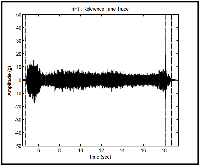
Figure description:
r(H : Reference Time Trace
r(H : Reference Time Trace
Annotations
- Boundary 1 (vertical_line - position: x = 4.8)
- Boundary 2 (vertical_line - position: x = 6.3)
- Boundary 3 (vertical_line - position: x = 18.1)
- Boundary 4 (vertical_line - position: x = 18.7)
| Time (sec) | Amplitude (g) |
|---|---|
| 4.0 | 0.0 |
| 4.5 | 0.0 |
| 4.8 | 1.0 |
| 4.8 | -1.0 |
| 5.0 | 10.0 |
| 5.0 | -12.0 |
| 5.5 | 15.0 |
| 5.5 | -18.0 |
| 6.0 | 11.0 |
| 6.0 | -13.0 |
| 6.3 | 5.0 |
| 6.3 | -6.0 |
| 7.0 | 6.0 |
| 7.0 | -6.5 |
| 8.0 | 8.0 |
| 8.0 | -8.5 |
| 9.0 | 9.0 |
| 9.0 | -9.0 |
| 10.0 | 8.0 |
| 10.0 | -8.0 |
| 11.0 | 7.5 |
| 11.0 | -7.5 |
| 12.0 | 8.5 |
| 12.0 | -8.5 |
| 13.0 | 9.5 |
| 13.0 | -9.5 |
| 14.0 | 7.5 |
| 14.0 | -7.5 |
| 15.0 | 6.5 |
| 15.0 | -6.5 |
| 16.0 | 7.0 |
| 16.0 | -7.0 |
| 17.0 | 8.0 |
| 17.0 | -8.0 |
| 18.0 | 10.0 |
| 18.0 | -15.0 |
| 18.1 | 5.0 |
| 18.1 | -5.0 |
| 18.4 | 4.0 |
| 18.4 | -4.0 |
| 18.7 | 1.0 |
| 18.7 | -1.0 |
| 19.5 | 0.0 |
Notes: The data points in the table represent the approximate envelope (peak and trough of the high-frequency time trace signal at specific intervals. Vertical dashed lines on the chart indicate significant transitions in the signal's characteristics.)
Figure 525.2A-5. Time trace segment identification from previously truncated reference time traces. The first and fifth segments represent low level pre- and post-test acceleration of no interest for test tolerance consideration. The second segment represents a transient vibration, the third segment stationary random vibration, and the fourth segment a shock. For further processing purposes, the three segments of interest are extracted by use of a rectangular window over the duration of the segment. The three segments are displayed in Figures 525.2A-6 through 525.2A-8.
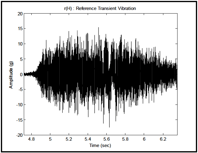
Figure description:
r(H : Reference Transient Vibration
r(H : Reference Transient Vibration
| Time (sec) | Min Amplitude (g) | Max Amplitude (g) |
|---|---|---|
| 4.70 | -0.5 | 0.5 |
| 4.80 | -1.0 | 1.0 |
| 4.85 | -3.0 | 3.5 |
| 4.90 | -6.0 | 8.5 |
| 5.00 | -10.0 | 11.5 |
| 5.10 | -12.5 | 13.0 |
| 5.20 | -14.0 | 14.5 |
| 5.30 | -13.5 | 14.0 |
| 5.40 | -13.0 | 13.5 |
| 5.50 | -14.5 | 15.5 |
| 5.60 | -16.0 | 13.0 |
| 5.65 | -17.5 | 11.0 |
| 5.70 | -15.0 | 11.5 |
| 5.80 | -11.5 | 13.0 |
| 5.90 | -9.0 | 11.5 |
| 6.00 | -8.5 | 10.5 |
| 6.10 | -7.5 | 9.0 |
| 6.20 | -6.5 | 8.0 |
| 6.30 | -5.0 | 6.0 |
| 6.35 | -4.0 | 5.0 |
Notes: The chart shows a high-frequency transient vibration signal. Due to the high density of data points, the provided table captures the upper and lower bounds (the envelope of the signal at sampled time intervals to represent its magnitude and duration accurately.)
Figure 525.2A-6. Transient vibration reference time trace segment.
MIL-STD-810H METHOD 525.2 ANNEX A
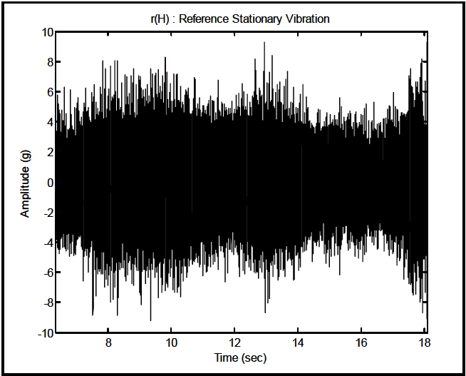
Figure description:
r(H : Reference Stationary Vibration
r(H : Reference Stationary Vibration
| Time (sec) | Amplitude (g) |
|---|---|
| 6.50 | 6.2 |
| 6.50 | -5.2 |
| 7.00 | 6.4 |
| 7.00 | -6.1 |
| 7.50 | 6.5 |
| 7.50 | -9.0 |
| 8.00 | 7.6 |
| 8.00 | -5.8 |
| 8.20 | 8.1 |
| 8.20 | -6.8 |
| 8.80 | 7.2 |
| 8.80 | -8.2 |
| 9.30 | 8.3 |
| 9.30 | -9.2 |
| 10.00 | 7.4 |
| 10.00 | -6.5 |
| 10.60 | 7.0 |
| 10.60 | -4.8 |
| 11.20 | 5.8 |
| 11.20 | -4.2 |
| 11.80 | 6.5 |
| 11.80 | -4.5 |
| 12.40 | 6.2 |
| 12.40 | -6.2 |
| 12.60 | 8.2 |
| 12.60 | -6.8 |
| 12.90 | 9.4 |
| 12.90 | -8.7 |
| 13.50 | 8.3 |
| 13.50 | -7.5 |
| 14.20 | 6.8 |
| 14.20 | -4.8 |
| 14.80 | 5.2 |
| 14.80 | -5.8 |
| 15.50 | 5.5 |
| 15.50 | -5.1 |
| 16.20 | 5.8 |
| 16.20 | -5.2 |
| 16.90 | 5.4 |
| 16.90 | -5.4 |
| 17.60 | 7.6 |
| 17.60 | -8.5 |
| 18.00 | 8.2 |
| 18.00 | -8.1 |
Notes: The chart represents a high-frequency stationary vibration signal. Due to the high density of the data points, the table captures representative peak and trough values to outline the signal's envelope and variation over time.
Figure 525.2A-7. Stationary random vibration reference time trace segment.
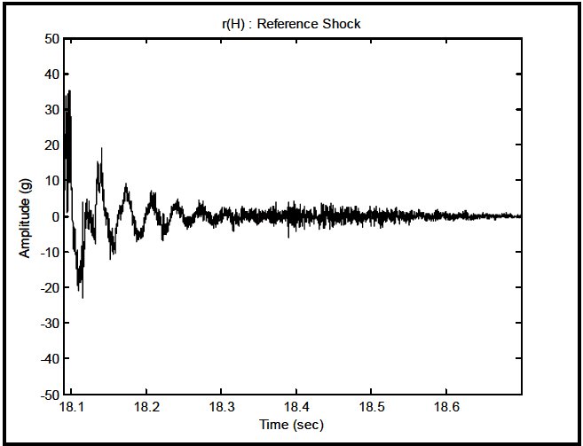
Figure description:
r(H : Reference Shock
r(H : Reference Shock
| Time (sec) | Amplitude (g) |
|---|---|
| 18.090 | 0.0 |
| 18.093 | 34.1 |
| 18.097 | 6.2 |
| 18.102 | 35.2 |
| 18.107 | -11.8 |
| 18.112 | -23.1 |
| 18.118 | 4.6 |
| 18.123 | 34.8 |
| 18.128 | -7.9 |
| 18.133 | 4.8 |
| 18.138 | 15.5 |
| 18.143 | 19.3 |
| 18.148 | -12.1 |
| 18.153 | -6.8 |
| 18.158 | 2.5 |
| 18.163 | 5.2 |
| 18.168 | 9.3 |
| 18.173 | -2.4 |
| 18.178 | -10.4 |
| 18.183 | -5.1 |
| 18.188 | 2.7 |
| 18.193 | 7.1 |
| 18.198 | -3.2 |
| 18.203 | -8.3 |
| 18.208 | -1.5 |
| 18.213 | 6.2 |
| 18.218 | -4.1 |
| 18.223 | -6.8 |
| 18.228 | 0.8 |
| 18.233 | 5.1 |
| 18.238 | -3.5 |
| 18.243 | -5.2 |
| 18.248 | 1.2 |
| 18.253 | 4.3 |
| 18.258 | -2.1 |
| 18.263 | -3.8 |
| 18.268 | 0.5 |
| 18.273 | 3.2 |
| 18.278 | -1.8 |
| 18.283 | -3.1 |
| 18.288 | 0.2 |
| 18.293 | 2.8 |
| 18.303 | -2.5 |
| 18.313 | 1.8 |
| 18.323 | -2.1 |
| 18.333 | 1.2 |
| 18.343 | -1.8 |
| 18.353 | 0.8 |
| 18.363 | -1.5 |
| 18.373 | 2.1 |
| 18.383 | -3.2 |
| 18.393 | -5.8 |
| 18.403 | 2.5 |
| 18.413 | 3.9 |
| 18.423 | -2.8 |
| 18.433 | 4.2 |
| 18.443 | -1.5 |
| 18.453 | 3.8 |
| 18.463 | -1.2 |
| 18.473 | 3.5 |
| 18.483 | -2.1 |
| 18.493 | 1.8 |
| 18.503 | -1.5 |
| 18.513 | 2.2 |
| 18.523 | -1.0 |
| 18.533 | 1.8 |
| 18.543 | -0.8 |
| 18.553 | 1.5 |
| 18.563 | -1.2 |
| 18.573 | 1.2 |
| 18.583 | -0.5 |
| 18.593 | 1.8 |
| 18.603 | -0.8 |
| 18.613 | 1.2 |
| 18.623 | -0.5 |
| 18.633 | 0.8 |
| 18.643 | -0.2 |
| 18.653 | 0.5 |
| 18.663 | 0.0 |
| 18.673 | 0.3 |
| 18.683 | -0.1 |
| 18.693 | 0.2 |
| 18.700 | 0.0 |
Notes: The chart represents a time-series of a shock signal, showing high-frequency oscillations that gradually decay over a period from approximately 18.09 seconds to 18.7 seconds. The vertical axis represents amplitude in g-units, ranging from -50 to 50, and the horizontal axis represents time in seconds.
Figure 525.2A-8. Shock reference time trace segment.
For materiel particularly sensitive to a band or bands of frequencies, both time traces may be filtered (phase linearity preserved) into a number of bands, and post-processing performed on the band or bands individually. It is quite acceptable to decide and agree upon (before laboratory testing) a band-pass filter strategy that will be acceptable for assessing replication error. This form replication error assessment will not be pursued further here.
MIL-STD-810H
METHOD 525.2 ANNEX A
4.5 Test Execution
4.5.1 Preparation for Test
Carefully examine the reference time trace for validity. Ensure the reference time trace is band limited according to the band limits of the exciter and control system software. By filtering, remove any high low-frequency components that will cause a displacement over-travel condition or velocity limit violation for the exciter. Make force requirement estimates based upon peak acceleration in the reference time trace, and the overall mass to be driven by the exciter, and compare this to the exciter force limits. If possible, integrate the acceleration time trace to obtain a velocity trace, and subsequently integrate the velocity trace to obtain a displacement trace to ensure the exciter is capable of reproducing the acceleration time trace without impacting its stops. Impacting stops, even in a cushioned hydraulic actuator, will typically result in materiel damaging accelerations. If integration is impractical or deemed likely inaccurate, the system may be operated using a dummy mass to determine if the available exciter stroke is sufficient. Generally, the vendor software estimates for maximum velocity and displacement should be verified, and some advanced signal processing procedures should be applied.
CAUTION: Integration is a difficult task that may provide unreliable answers. Using a technique such as a wavelet transformation, recommend removal of DC bias or very low frequency drift that falls below the minimum frequency of interest without imposing a phase lag.
4.5.1.1 Preliminary Steps
Deciding upon the strategy for TWR compensation of the reference time trace, i.e., determining the exciter drive voltage, is a very important and potentially time-consuming task. The vendor approach to reference time trace compensation must be clearly understood. The advantages and disadvantages of time and frequency compensation error reduction strategies must be clearly understood. Boundary conditions and impedance mismatches almost always require maximum use of all the vendor software strategies for compensation. Use of exciter slip tables present special challenges for reference time trace compensation. Vendor software will generally allow compensation on (1) a band limited random signal, (2) a reduced level of the reference time trace, or (3) the full level reference time trace as the test progresses or as accumulated from previous testing at full level. Some vendor software may allow different compensation functions (transfer functions) on different portions of the reference time trace. It is recommended that testing be initially performed on a dynamic simulant item that represents the dynamic properties of the materiel to be tested to ensure the reference time trace can be properly compensated and accurately replicated. Remember that the bandwidth of the control time trace reflects the response of the dynamic simulation item or the materiel, and may be substantially broader than the bandwidth of the reference time trace. TWR “control” is generally active only over the bandwidth of the reference time trace, allowing uncompensated response outside of this bandwidth. Vendor software may permit control beyond the band limit of the reference time trace. If the bandwidth differences (reference versus control) can be detected early on, this will be helpful in interpreting the results of the test, particularly with respect to meeting test tolerances.
MIL-STD-810H
METHOD 525.2
4.5.1.2 Pretest Checkout
Verify that each of the following check list items is established prior to initiation of the test
- a. Test fixture requirements.
- b. Test fixture modal survey requirements / procedure.
- c. Test item/fixture modal survey requirements / procedure.
- d. Control and monitor measurement locations correlate with the configuration for which the reference time trace was obtained.
- e. Test tolerances.
- f. Requirements for combined environments.
- g. Test schedule(s) and duration of exposure(s).
- h. Axes of exposure.
- i. Test shutdown procedures for test equipment or test item problems, failures, etc.
- j. Test interruption recovery procedure. (See paragraph 4.3.)
- k. Test completion criteria including any post processing for a refined tolerance assessment (STTR).
- Test requirements (force, acceleration, velocity, displacement) can be met. Seek approval for variation if required. Document any variation.
- m. Allowable adjustments to test item and fixture (if any); these must be documented in test plan and the test report.
- n. Adequate digital data storage requirements.
4.5.2 Procedure Specific
The following steps provide the basis for collecting the necessary information under TWR testing.
4.5.2.1 Procedure I - SESA Replication of a Field Measured Materiel Time Trace Input/Response
- Step 1 Following the guidance of paragraph 6.1, reference b, select the test conditions and mount the test item (or dynamic simulant item) on the vibration exciter. Select accelerometers and analysis techniques that meet the criteria outlined in paragraph 6.1, reference b.
- Step 2 If required; perform an operational check on the test item at standard ambient conditions. If the test item operates satisfactorily, proceed to Step 3. If not, resolve the problems and repeat this step.
- Step 3 Subject the test item (or dynamic simulant) to the system identification process that determines the compensated exciter drive voltage. This may include a careful look at the component parts of the reference time trace, i.e., stationary vibration, shock, transient vibration; and determination of the potential time variant properties of the compensating function. If a dynamic simulant is used, then replace the dynamic simulant with the test item after compensation.
- Step 4 Subject the test item in its operational configuration to the compensated waveform. It is often desirable to make an initial run at less than full level to ensure proper dynamic response and validate instrumentation functionality.
- Step 5 Record necessary data, paying particular attention to the vendor software supplied test error indicator and, in general, the control acceleration time trace that can be post processed to demonstrate tolerance satisfaction.
- Step 6 Perform an operational check on the test item and record the performance data as required. If failure is noted, follow the guidance in paragraph 4.3.2.
- Step 7 Repeat Steps 4, 5, and 6 for the number of replications called out in the requirements document, or a minimum of three times for statistical confidence provided the integrity of the test configuration is preserved during the test.
Step 8 Document the test series including the saving of all control and monitor digital time traces, and see paragraph 5 for analysis of results.
4.5.2.2 Procedure II - SESA Replication of an Analytically Specified Materiel Time Trace Input/Response
Follow the guidance provided in Steps 1-8 in Paragraph 4.5.2.1 subsequent to scaling the reference time trace per the scaling guidance provided in paragraph 1.2.6.
4.5.3 Data Analysis
Ideally, information from the control time trace in the time and frequency domains should be nearly identical to that information contained in the reference time trace. Vendor supplied test error assessment provides a preliminary indication of the replication efficacy. If vendor supplied test error assessment consistently displays less than, e.g., 5 percent time average rms error over blocks of reference/control data, additional analysis may be unnecessary. For production testing, reliance on consistency of vendor supplied rms error is highly desirable. For single item tests that are unique and for which vendor rms error provides values greater than acceptable, then differences between the reference and control time traces must be assessed in detail. The following guidance is provided.
- a. Rudimentary analysis to ensure the test tolerances are met is usually performed within the TWR vendor software. Laboratory personnel should consult the vendor supplied TWR system documentation, and clearly understand the determination of these test tolerances. In most cases, this will require direct contact with the vendor of the TWR system.
- b. More extensive data analysis can be performed to ensure test tolerances are met based upon reference and control time trace ASCII files, with off line specialized software according to procedures illustrated in Annex A and discussed in Annex B.
- c. Detailed data analysis for purposes of establishing parameters for a random process or other purposes may be performed, but must be consistent with the information provided in the Annexes, and best data processing procedures as defined in paragraph 6.1, references a or b. Such detailed analysis may be beyond the scope of defined tolerances, and is to be used for report information purposes only.
- d. Processing of monitor time trace information for modeling, failure assessment, or other purposes must follow the same guidelines as for the control time trace.