528.1-5 SUPERSEDING DATA
This Method covers Types I and II vibration requirements formerly covered in MIL-STD-167-1 & 1A (SHIPS). Types III, IV, and V requirements are covered in MIL-STD-167-2A (SH).
MIL-STD-810H METHOD
528.1-5 ADDITIONAL ENVIRONMENTAL ELEMENTS
Several additional climatic or other environmental elements are known to have effects on some kinds of military materiel. The elements are discussed in the following paragraphs and, where possible, operational extremes are given.
5.1 Procedure I (Type I) – Environmental Vibration
When Type I vibration requirements are specified (see Annex B, paragraph 2e), the test item shall be subjected to a simulated environmental vibration as may be encountered aboard Naval ships. This Method provides an amplitude sufficiently large within the selected frequency range to obtain a reasonably high degree of confidence that equipment will not malfunction during service operation.
- a. For Type I vibration testing, this Method shall be used for equipment subjected to the vibration environment found on Navy ships with conventionally shafted propeller propulsion.
- b. For Type I vibration testing this Method can be tailored for non-conventional Navy shafted propeller systems such as waterjet, poded, or other propulsor types, including those that have been designed to minimize blade-rate forces. The revised test Method shall be recommended by the purchaser and approved by the Government.
- c. For equipment installed on ships with propulsion systems with frequency ranges not covered by Table 528.1-I, this Method shall not apply.
528.1-5.1 Wind
5.1.1 Basis of Acceptability
For equipment that can be vibration tested, acceptability shall be contingent on the ability of the equipment to withstand tests specified, and the ability to perform its principal functions during and after vibration tests. Minor damage or distortion will be permitted during the test, providing such damage or distortion does not in any way impair the ability of the equipment to perform its principal functions (see Annex B, paragraphs 2f(1) and 2f(6)). Because of the numerous types of equipment covered by this Method, a definite demarcation between major and minor failures cannot be specified. Therefore, during testing acceptability a determination shall be made as to whether or not a failure
MIL-STD-810H
METHOD 528.1
is minor or major to determine whether testing should continue (see Annex B, paragraph 2f(2)). In general, a major failure is one that would cause mal-operation or malfunction of the item of equipment for a long period. Non-repetitive failures of such parts as connectors, knobs/buttons, certain fasteners, and wiring, that can be easily replaced or repaired, are generally considered minor failures. As such, the repair could be made and the test continued with no penalty to the remainder of the test item. The critical use of the equipment shall be considered when determining the category of failure; e.g., a failure of a part in a lighting circuit may be considered minor. The same failure in a control circuit may be major.
528.1-5.1.1 Wind element
Wind is probably the most complex of all climatic elements affecting materiel. Wind effects are difficult to analyze because wind is a vector quantity subject to rapid temporal and spatial changes in speed and direction. In addition to parameters of average speed and direction, a complete description of wind includes the random motions of widely different scales, and periods called “atmospheric turbulence” or “eddies.” The wind forces on a structure result from differential pressures, positive and negative, caused by an obstruction to the free flow of the wind. Thus, these forces are functions of the velocity and turbulence of the wind and of the orientation, area, and shape of the elements of the structure.
- a. For operations, the following extremes, as given in MIL-HDBK-310, are: a steady wind speed of 22 m/s (49.2 mph) and a gust of 29 ms (65 mph).
- b. The above operational wind speeds are for a height of 3m (10 feet). Multiplication factors for obtaining speeds at the height of materiel are shown in Table XII.
Table XII. Wind speed multiplication factors at selected heights
| Height | Operational | ||
|---|---|---|---|
| Meters | Feet | Steady winds | Gusts |
| 1.5 | 0.5 | 0.917 | 0.946 |
| 3 | 10 | 1.000 | 1.000 |
| 6 | 20 | 1.090 | 1.057 |
| 9 | 30 | 1.147 | 1.092 |
| 12 | 40 | 1.189 | 1.117 |
| 15 | 50 | 1.222 | 1.137 |
| 23 | 75 | 1.286 | 1.175 |
| 30 | 100 | 1.334 | 1.202 |
| 61 | 200 | 1.454 | 1.271 |
| 91 | 300 | 1.510 | 1.313 |
| 122 | 400 | 1.586 | 1.343 |
| 152 | 500 | 1.631 | 1.368 |
| 305 | 1000 | 1.778 | 1.445 |
5.1.2 Test Procedures
The tests specified herein are intended to expose equipment to:
- a. Vibration magnitudes in prescribed frequency and amplitude ranges to reveal any critical response prominences (see paragraph 2.2v) or potential deficiencies.
- b. A 2-hour minimum endurance test at the response prominence frequency or frequencies most seriously affecting its functional or structural integrity.
528.1-5.1.2 Wind speed
Observations of wind speed are one of the least standardized of all meteorological elements. The exposure and height above the ground of wind-measuring materiel is far from uniform. Because wind speeds near the ground can vary significantly with height and exposure, specifying this variability is an important problem. Another problem is that the interval over which wind speeds are averaged, varies from country to country. The current standard averaging period in the United States, 1 min, is considered representative of the values herein referred to as the "average or steady wind." Gusts associated with steady wind speeds must also be considered.
The gust factor is the ratio of the gust speed to the steady wind speed. Although many factors influence this ratio, one can develop approximations for the gust factor as a function of steady wind speed. Gust speeds reported in weather observations are normally considered to be about 3-sec averages, but for designing various sized materiel, other short-duration gusts are often applicable. A previous study indicates that a gust must have a duration such that its size is about eight times the downwind dimension of a structure in order to produce a force on the structure commensurate with the gust speed. For example, a structure with a 3m (10 ft) downwind dimension must have a 24m (79 ft) long gust to establish full dynamic pressure on the structure. Smaller structures will be sensitive to shorter-duration gusts.
The most probable gust extremes associated with the 1-min steady extremes presented in the following sections are scaled to arbitrarily chosen downwind materiel dimensions of 0.6, 1.5, 3, 8, 15, and 30m (2, 4.9, 10, 26, 49, and 98 ft). Because the placement of most materiel will not take into consideration the direction of the extreme wind speeds, consider the shortest horizontal dimension of the materiel as the downwind dimension.
MIL-STD-810H
PART THREE
- a. Highest Recorded. The highest recognized worldwide maximum wind speed measured at a surface station is a 5-minute speed of 177 knots (204 mph), and a 1-second gust of 196 knots (226 mph) measured at Mt. Washington Observatory, New Hampshire, on 12 April 1934. The Observatory is 1915m (6280 ft) above MSL, and the anemometer was mounted at 12m (39 ft). However, this is an anomalous location, and such values should not be considered for this standard.
Tornado winds also are excluded from consideration because they are considered to be too localized. No wind measuring device has ever survived the full fury of a tornadic wind. Authorities have suggested that the winds could exceed 350 knots (403 mph).
A 152 knot (175 mph) gust at a height of 9.2m (30 ft) (corresponding to 139 knots (160 mph) at 3m (10 ft)) was recorded during a typhoon that passed over Iwo Jima AB, Volcano Islands in the Pacific Ocean in 1948. The maximum sustained wind is a 5-min speed of 131 knots (151 mph) measured at a height of 16.5m (54 ft) (corresponding to 119 knots (137 mph) when corrected to a 1-minute speed at 3m) at San Juan, Puerto Rico. These two extremes should not be considered as the highest winds that have occurred over a general area or region. Certainly, higher speeds have occurred, but have not been recorded due to their devastating damage.
The highest wind speeds affecting sizable areas occur within the typhoons that pass over the islands of the western North Pacific Ocean. Of these, Typhoon Nancy, during the period 11-12 September 1961, was the most intense typhoon ever observed by the Joint Typhoon Warning Center (Inception date for the JTWC was 1945). They reported maximum surface winds to be 185 knots (213 mph), estimated from air reconnaissance observations. For this standard, it is assumed that the highest sustained wind-speeds affecting a sizable area of military concern was the 185 knots (213 mph) (sustained for a duration of several minutes). The most probable 2-second gust to accompany this sustained wind is estimated to be 204 knots (235 mph).
b. Frequency of Occurrence. The location having the highest 1-percent wind is Northern Scotland. Typical of the area is Stornoway where in the windiest month (December), the 1-, 5- and 10-percent high wind speeds are 43, 36 and 33 knots (49.5, 41.4, and 38 mph), respectively (1-min speeds at a 3m (10 ft) height). The most probable gusts that can be expected to accompany these 1-, 5- and 10-percent wind speeds, based on the shortest horizontal dimension of the materiel, are given in the following table:
Table XIII. Associated gusts (m/s (mph)).
| Percent Extreme | 1-min Steady m/s (mph) | Shortest Horizontal Dimension of Materiel (m (ft)) | |||||
|---|---|---|---|---|---|---|---|
| <0.6 (2) | 1.5 (4.9) | 3 (9.8) | 8 (26) | 15 (49) | 30 (98.4) | ||
| 1 | 22 (49.5) | 32 (71.6) | 59 (132) | 56 (125.3) | 53 (118.6) | 50 (112) | 48 (107.4) |
| 5 | 19 (41.4) | 27 (60.4) | 49 (109.6) | 47 (105) | 44 (98.4) | 42 (94) | 40 (89.5) |
| 10 | 17 (38) | 25 (56) | 45 (100.7) | 43 (96.2) | 40 (89.5) | 38 (85) | 36 (80.5) |
Note: Most meteorological reports give wind speed in knots; 1 knot = 1.15 mph; 1 knot = 0.51 m/s. The wind speeds in Table XIII are for a height of 3m (10 ft). Speeds can be estimated for other heights by using power law relationship
where is the velocity at the desired height, is the velocity at 3 m, z is the desired height in meters, and P is an exponent that varies primarily with terrain and stability. MIL-STD-210B used P values of 0.125 for winds less than 50 kts (58 mph) and 0.08 for gusts and winds of at least 50 kts (58 mph). However, this resulted in circumstances where the steady speeds exceeded the gusts. Therefore, a compromise of
is recommended for converting these wind speeds and gusts to other heights up to 100m (328 ft). Reference to more detailed information is provided in Annex A.
c. Long-term Extremes
The area having the highest winds in the world (excluding mountain peaks and tornado tracks) is in the typhoon belt of the western North Pacific Ocean. (This area ordinarily has relatively low wind speeds). Locations typical of the center of this belt are the Volcano Islands (for example, Iwo Jima) and Ryukyu Islands (for example, Okinawa). Of these locations, Naha, Okinawa (26°12'N, 127°39'E, station elevation 7m (23 ft) MSL) was found to have the highest annual extremes. Based on 19 years of data, long term extremes were computed. The mean of the highest annual 2-sec gusts is 84 knots (97 mph) with a standard deviation of 26.4 knots (30 mph). Applying these statistics in the theory of extremes, the 2-sec gusts that can be expected to occur at least once during 10, 30, and 60 yrs are 134, 154, and 167 kts (154, 177, and 192 mph) respectively. The most probable 1- min steady winds associated within these 2-sec gusts are 119, 140, and 156 kts (137, 161, and 180 mph) respectively. Gusts for various shortest horizontal dimensions of materiel are presented in the following table:
Table XIV. Associated gusts (m/s (mph)).
| Period (yrs) | 1-min Steady Speed m/s (mph) | Shortest Horizontal Distance of Materiel (m (ft)) | |||||
|---|---|---|---|---|---|---|---|
| <0.6 (2) | 1.5 (4.9) | 3 (9.8) | 8 (26) | 15 (49) | 30 (98.4) | ||
| 10 | 61 (136.5) | 77 (172) | 74 (166.5) | 73 (163.3) | 71 (158.8) | 69 (154.3) | 68 (152) |
| 30 | 72 (161) | 87 (194.6) | 85 (190) | 83 (185.7) | 81 (181.2) | 80 (179) | 78 (174.5) |
| 60 | 80 (179) | 95 (212.5) | 93 (208) | 91 (203.6) | 89 (199) | 88 (196.9) | 86 (192.4) |
Note: Most meteorological reports give wind speed in knots; 1.15 mph = 1 knot; 1 m/s = 1.94 knot.
These wind speeds are for a height of 3m (10 ft). Speeds (and gusts) can be estimated for other heights up to 100m (328 ft) by using the power law relationship in paragraph 5.1.2b, with a value of 0.08 for P. This lower value for P is recommended because these extremely high wind speeds occur in open areas where winds decrease less rapidly with height.
5.1.2.1 Testing Machine
Vibration tests shall be made by means of any testing machine capable of meeting the conditions specified in paragraph 5.1.2.4, and the additional requirements contained herein. Means shall be provided for controlling the direction of vibration of the testing machine, and for adjusting and measuring its frequencies and the amplitude of vibration to keep them within prescribed limits. It is acceptable to use different machines for the vertical and horizontal directions. The testing machine, including table, actuator, and attachment fixtures, shall be rigid within the frequency range to be tested. This includes test fixture resonances that may result from interaction between the table and mounted test items. Testing machine rigidity shall be demonstrated by analysis, or by measuring transmissibility in accordance with paragraph 5.1.2.2d.
5.1.2.2 Additional Test Instrumentation
Vibration measurement transducers such as accelerometers shall be installed on the test item to aid in the determination of response prominences during the exploratory and variable frequency vibration tests of paragraphs 5.1.2.4.2 and 5.1.2.4.3. The number, orientation, and placement of vibration transducers will depend upon the equipment under test, and should be sufficient to provide a suitable survey for identifying response prominences of the tested equipment and testing machine. When required, approval of transducer locations shall be obtained from the procuring activity (see Annex B, paragraph 2f(3)). Guidance below shall be used in the selection of measurement locations:
- a. Measurements shall be made at locations corresponding to components or areas on the equipment of particular concern for operation of the equipment, whose failure would impair the ability of the equipment to perform its principal function. Such locations shall be determined prior to test.
- b. Select a sufficient number of measurement locations such that the response of the test item is measured at locations near the base, top, and center of the test item to measure response prominences associated with global motion of the equipment. Attach these transducers to rigid areas of the test item representing major structural components such as the housing, shell, or body of the equipment.
- c. The transducers shall be oriented to measure vibration in the direction of the vibration excitation provided for any given test. If necessary, transducers may be re-oriented between tests.
- d. If the testing machine rigidity has not been demonstrated by analysis, a sufficient number of transducers shall be located on the testing machine to demonstrate that the testing machine is rigid over the frequency range of the test. At a minimum, locate these transducers at the point of force application to the table, and at the test item attachment interface(s) to the testing machine.
5.1.2.3 Methods of Attachment
5.1.2.3.1 Shipboard Equipment
For all tests, the test item shall be secured to the testing machine at the same points or areas of attachment that will be used for securing it shipboard. In case alternate attachment points or areas are specified, tests shall be performed using each attachment configuration. Equipment that is hard mounted (i.e., not isolation mounted) aboard ship shall be hard mounted to the testing machine. For equipment designed to be secured to a deck and a head brace support, a vertical
MIL-STD-810H
METHOD 528.1
bracket shall be used to simulate a bulkhead. The bracket shall be sufficiently rigid to ensure that its motion will be essentially the same as the motion of the platform on the testing machine. For isolation mounted shipboard equipment, see paragraph 5.1.2.3.4.
5.1.2.3.2 Shipboard Portable and Test Equipment
Portable and test equipment that is designed for permanent or semi-permanent attachment to a ship structure shall be attached to the vibration testing machines in the same manner it is attached to the ship. Equipment that is not designed for permanent or semi-permanent attachment shall be secured to the testing machine by suitable means.
5.1.2.3.3 Orientation for Vibration Test
Test items shall be installed on vibration testing machines in such a manner that the direction of vibration will be, in turn, along each of the three rectilinear orientation axes of the equipment as installed on shipboard – vertical, athwartship, and fore and aft. On a horizontal vibration-testing machine, the test item may be turned 90 degrees in the horizontal plane in order to vibrate it in each of the two horizontal orientations. At no time shall the test item be installed in any other way than its normal shipboard orientation.
5.1.2.3.4 Isolation Mountings
For Type I testing of equipment to be installed shipboard on isolation mounts, testing shall be performed on isolation mounts or hard mounted to the testing machine, or as specified (see Annex B, paragraph 2f(4)). Type I testing of a particular test item on isolation mounts is valid only for the isolation mount type and configuration used during testing. Ensure the transmissibility across the mounts does not exceed 1.5 within the blade frequency range of 80 percent to 115 percent of design RPM. If equipment is tested for Type I vibrations hard mounted to the test fixture throughout the duration of the test, the test is valid for either hard mounted or isolation mounted shipboard installations, provided the isolation mounts are Navy standard mounts contained in MIL-M-17191, MIL-M-17508, MIL-M-19379, MIL-M-19863, MIL-M-21649, MIL-M-24476 (see paragraph 6.1, references a-f), or distributed isolation equipment (DIM).
5.1.2.3.5 Internal Isolation or Shock Mountings
Equipment that incorporates other isolation mountings integrally within the equipment box (such as electronic cabinets) shall be tested with the internal mountings in the normal shipboard configuration or as specified (see Annex B, paragraph 2f(5)).
5.1.2.4 Vibration Tests
Each of the tests specified shall be conducted separately in each of the three principal directions of vibration. All tests in one direction shall be completed before proceeding to tests in another direction. The test item shall be secured to the vibration table as specified in paragraph 5.1.2.3. If major damage occurs (see paragraphs 4.3 and 5.1.1), the test shall be discontinued, and the entire test shall be repeated following repairs or correction of deficiencies.
5.1.2.4.1 Equipment Operation
Except as noted below, the test item shall be energized or operated to perform its normal functions (see Annex B, paragraph 2f(6)). Equipment that is difficult to operate on the testing machine shall be energized and subjected to operating conditions during the test. The test item shall then be operated after the test to demonstrate that there is no damage from the test (see Annex B, paragraph 2f(1)).
5.1.2.4.2 Exploratory Vibration Test
To determine the presence of response prominences (see paragraph 2.2v) in the test item, it shall be secured to the vibration table and vibrated at frequencies from 4 Hz to 33 Hz, at a table vibratory single amplitude of 0.010 ± 0.002 inch (see paragraphs 5.1.2.4.4 and 5.1.2.4.5 for exceptions). The change in frequency shall be made in discrete frequency intervals of 1 Hz, and maintained at each frequency for about 15 seconds. Alternatively, a continuous frequency sweep with a rate of change of frequency not to exceed 0.067 Hz/second can be used. The frequencies at which functional or structural requirements are affected or violated and frequencies and locations at which response prominences occur shall be recorded, and these frequencies (rounded to the nearest integer frequency if discrete frequency intervals were not used) shall be considered as candidates for endurance testing (see Annex A).
MIL-STD-810H
METHOD 528.1
5.1.2.4.3 Variable Frequency Test
The test item shall be vibrated from 4 Hz to 33 Hz in discrete frequency intervals of 1 Hz, and at the amplitudes shown in Table 528.1-I (see paragraphs 5.1.2.4.4 and 5.1.2.4.5 for exceptions). At each integral frequency, the vibration shall be maintained for 5 minutes. The frequencies, at which functional or structural requirements are affected or violated, and frequencies and locations at which response prominences occur, shall be recorded. Note that because of increased amplitudes compared to those in paragraph 5.1.2.4.2, response prominences and effects on or violations of functional or structural requirements may show up in this test that were not uncovered in the exploratory vibration test. Therefore, the frequencies at which these response prominences and effects on or violations of functional or structural requirements occur shall also be considered as candidates for endurance testing (see Annex A).
| Frequency range (Hz) | Table single amplitude (inch) |
|---|---|
| 4 to 15 | 0.030 ± 0.006 |
| 16 to 25 | 0.020 ± 0.004 |
| 26 to 33 | 0.010 ± 0.002 |
5.1.2.4.4 Exception
Equipment intended for installation solely on a particular ship class need only be vibrated in the exploratory and variable frequency tests from 4 Hz to (1.15 x design rpm x number of propeller blades/60) rounded up to the nearest integer frequency or the maximum test frequency as specified by the purchaser and approved by the Government.
5.1.2.4.5 Alternative Test Amplitudes
For equipment installed on ships with advanced isolation systems, low vibration propellers, or other reduced environment vibration conditions, the alternative test amplitudes can be reduced. A reduction in test amplitude shall be recommended by the purchaser and approved by the Government.
5.1.2.4.6 Endurance Test
Endurance test frequencies are selected from the candidate list of endurance test frequencies developed during exploratory and variable frequency testing (see paragraphs 5.1.2.4.2 and 5.1.2.4.3). When specified (see Annex B, paragraph 2f(9)), selection of these frequencies is subject to approval. The test item shall be vibrated for a total period of at least 2 hours at the frequency determined to most seriously affect the functional or structural integrity of the equipment. Guidance for selecting response prominences from exploratory or variable frequency testing, for determining whether a response prominence is significant, and if the more serious response prominences can be identified, is given in Annex A. In cases where there are multiple response prominence frequencies selected, the duration of vibration testing at each frequency shall be in accordance with Table 528.1-II. If neither response prominences nor effects on equipment structural/functional performance are observed, this test shall be performed at 33 Hz or at the upper frequency as specified in paragraph 5.1.2.4.4. Ensure the amplitudes of vibration are in accordance with Table 528.1-I, unless otherwise specified (see paragraph 5.1.2.4.5). See Figure 528.1-1 for a graphical representation of the amplitudes in Table 528.1-I.
MIL-STD-810H
METHOD 528.1
| Number of endurance test frequencies | Test time duration at each endurance test frequency | Total time |
|---|---|---|
| 1 | 2 hours | 2 hours |
| 2 | 1 hour | 2 hours |
| 3 | 40 minutes | 2 hours |
| 4 | 40 minutes | 2 hours, 40 minutes |
| n>2 | 40 minutes | 40 x n minutes |
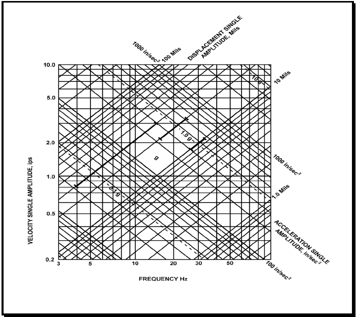
Figure description:
Vibration Frequency-Amplitude Relationship Chart
Vibration Nomograph
Legend
- Velocity Single Amplitude (ips — color: black; symbol: Vertical axis
- Frequency (Hz — color: black; symbol: Horizontal axis
- Displacement Single Amplitude (Mils — color: black; symbol: Positive slope diagonals
- Acceleration Single Amplitude (in/sec² — color: black; symbol: Negative slope diagonals
- Specific vibration profile — color: black; symbol: Bold line segments
Annotations
- 1.0 g (text_label - position: Diagonal line sloping downward from left to right, highlighted with tick marks)
- 0.1 g (text_label - position: Dashed diagonal line below 1.0 g line)
- 10 g (text_label - position: Dashed diagonal line above 1.0 g line)
- g (text_label - position: Centered in diamond-shaped grid area)
| Series | Frequency (Hz) | Velocity (ips) | Displacement (Mils) | Acceleration (in/sec²) |
|---|---|---|---|---|
| Displacement 1.0 Mil | 31.83 | 0.20 | 1.0 | 40.0 |
| Displacement 1.0 Mil | 100.00 | 0.628 | 1.0 | 394.8 |
| Displacement 10 Mils | 3.18 | 0.20 | 10.0 | 4.0 |
| Displacement 10 Mils | 10.00 | 0.628 | 10.0 | 39.5 |
| Displacement 10 Mils | 100.00 | 6.283 | 10.0 | 3948.0 |
| Displacement 100 Mils | 3.00 | 1.885 | 100.0 | 35.5 |
| Displacement 100 Mils | 15.92 | 10.00 | 100.0 | 1000.0 |
| Acceleration 100 in/sec² | 3.00 | 5.305 | 281.4 | 100.0 |
| Acceleration 100 in/sec² | 79.58 | 0.20 | 0.4 | 100.0 |
| Acceleration 1000 in/sec² | 15.92 | 10.00 | 100.0 | 1000.0 |
| Acceleration 1000 in/sec² | 100.00 | 1.592 | 2.5 | 1000.0 |
| Acceleration 0.1 g | 3.00 | 2.048 | 108.7 | 38.6 |
| Acceleration 0.1 g | 30.73 | 0.20 | 1.0 | 38.6 |
| Acceleration 1.0 g | 6.15 | 10.00 | 258.9 | 386.1 |
| Acceleration 1.0 g | 61.45 | 1.00 | 2.6 | 386.1 |
| Acceleration 1.0 g | 100.00 | 0.615 | 1.0 | 386.1 |
| Acceleration 10 g | 61.45 | 10.00 | 25.9 | 3861.0 |
| Bold Profile | 4.00 | 0.83 | 33.0 | 20.9 |
| Bold Profile | 14.50 | 3.00 | 33.0 | 273.6 |
| Bold Profile | 20.50 | 3.00 | 23.3 | 387.0 |
| Bold Profile | 31.00 | 1.98 | 10.2 | 386.1 |
Notes: The chart is a four-way logarithmic nomograph relating frequency (Hz, velocity (ips, displacement (mils, and acceleration (in/sec². The bold lines define a specific vibration envelope consisting of a constant displacement segment (33 mils, a constant velocity segment (3.0 ips, and a constant acceleration segment (1.0 g. The values for g are based on standard gravity ≈ 386.1 in/sec².)))))))
Figure 528.1-1. Type I environmental vibration limits (black bars represent a graphical presentation of Table 528.1-I expressed in displacement, velocity, and acceleration)
5.1.2.4.7 Endurance Test for Mast Mounted Equipment
Equipment intended for installation on masts, such as radar antennae and associated equipment, shall be designed for a static load of 2.5g (1.5g over gravity) in vertical and transverse (athwartship and longitudinal) directions to compensate for the influence of rough weather. In addition, the test item shall be vibrated for a total period of at least 2 hours at the response prominences chosen by the test engineer. When specified (see Annex B, paragraph 2f(9)), selection of these frequencies is subject to approval. If no response prominences were observed, this test shall be performed at 33 Hz, unless excepted by paragraph 5.1.2.4.4, in which case use the maximum frequency specified in paragraph 5.1.2.4.4 shall be used. The amplitudes of vibration shall be in accordance with Table 528.1-III.
MIL-STD-810H
METHOD 528.1
| Frequency Range (Hz) | Table Single Amplitude (inch) |
|---|---|
| 4 to 10 | 0.100 ± 0.010 |
| 11 to 15 | 0.030 ± 0.006 |
| 16 to 25 | 0.020 ± 0.004 |
| 26 to 33 | 0.010 ± 0.002 |
5.1.2.5 Test Documentation
5.1.2.5.1 Test Plan
When specified (see Annex B, paragraph 2b), an equipment test plan shall be prepared for Type I tests in accordance with DI-ENVR-81647 (see Annex B, paragraph 3). The test plan shall specify, describe, or define all requirements, and shall be approved by the acceptance authority prior to the test as specified (see Annex B, paragraph 2f(10)).
5.1.2.5.2 Test Report
A test report (see Annex B, paragraph 2b) for Type I tests shall be prepared in accordance with DI-ENVR-81647 (see Annex B, paragraph 3), and shall be approved by the acceptance authority as specified (see Annex B, paragraph 2f(10)).
5.1.3 Exemption
If equipment size, weight, or center-of-gravity precludes testing on existing vibration facilities, the test item may be qualified by analysis or individually testing integral parts of the equipment, as approved by the acceptance authority. To facilitate this analysis process, the equipment could be shock tested to determine the natural frequencies. If the measured frequencies do not clear the blade rate by 25 percent, the equipment should be stiffened, and thereby, its vibration resistance increased.
5.1.4 Extension of Previous Testing
Equipment that is identical or similar to previously tested equipment may qualify for an extension of the previously approved test. The equipment for which the testing is to be extended must meet all of the following criteria:
- a. The tested equipment and the proposed extension equipment are made of the same or similar equipment, and manufactured using the same or similar processes.
- b. The mass of the proposed extension equipment is no more than 10 percent greater than the mass of the tested equipment.
- c. The location of the center of gravity of the proposed extension equipment is within 10 percent of the location of the center of gravity of the tested equipment.
5.1.4.1 Extension Documentation
A request for extension of previously approved testing must be approved by the acceptance authority and must contain the following:
- a. Detailed drawings of both the tested equipment and proposed extension equipment.
- b. A copy of the test report for the tested equipment.
- c. A detailed comparison of the differences in equipment and design showing that the proposed extension equipment has equal or greater vibration resistance than the tested equipment. This comparison should include at a minimum the information requested in paragraphs 5.1.4a, b, and c.
MIL-STD-810H
METHOD 528.1
5.1.5 Alignment Criteria
- a. Equipment foundations should be such that they are devoid of natural frequencies within 25 percent of blade rate. If this guideline is not met, alignment issues will arise. That is, a tracker will not be able to home in on a target.
- b. Equipment foundation response should not exceed 1/7th of the vibration displacement of environmental vibration. For combatants with an alternating thrust between +1 and +1.5 percent, Standardization Activity SH (NAVSEA 05P12) can allow a response of up to 2/7ths. If this guideline is not met, alignment issues can arise.
- c. In order to reduce tracker alignment issues, a 57 mm gun, for example, should be designed with a total foundation impedance of 400 lb sec/in.
- d. Superstructure deck response should not exceed 1/7th of vibratory displacement of environmental vibration for the mast mounted equipment. If this guidance is not met, the tracker can lose control with the satellite.
5.2 Procedure II (Type II) – Internally Excited Vibration
Unless otherwise specified (see Annex B, paragraph 2e), Type II balance and vibration requirements shall apply to the procurement of rotating machinery. This does not apply to suitability from a noise standpoint, nor does it apply to reciprocating machinery. Special vibration and balance requirements may be specified (see Annex B, paragraph 2g(1)). The limitations set forth herein may also be used as criteria on overhaul tolerances, but should not constitute a criterion for the need for overhaul.
528.1-5.2 Rain
5.2.1 Basis of Acceptability
All rotating machinery shall be balanced to minimize vibration, bearing wear, and noise. Types of balancing shall be as specified in Table 528.1-IV. Machinery with rigid rotors shall meet the limits of allowable residual unbalance given in paragraph 5.2.2.2. For machinery with rotors that are unable to meet the balance requirements of rigid rotors, shall be balanced in accordance with the requirements of paragraph 5.2.3.1.
NOTE: The pitch of each propeller blade should be the same. If this is not the case, the added mass on the propeller blades will be different, and the propeller will be unbalanced.
| Rotor Characteristics | Speed (rpm) | Type of Balancing | Balancing Methods and Limits |
|---|---|---|---|
| Rigid, L/D 1/ ≤0.5 | 0-1000 | Single-plane | 5.2.2 |
| >1000 | Two-plane | 5.2.2 | |
| Rigid, L/D>0.5 | 0-150 | Single-plane | 5.2.2 |
| >150 | Two-plane | 5.2.2 | |
| Flexible | All | Multi-plane (more than two planes) | 5.2.3 |
L - Length of rotor, exclusive of shaft.
D – Diameter of rotor, exclusive of shaft.
528.1-5.2.1 Intensities
The world's highest rainfall intensities are in areas that experience the constant high humidity conditions of the basic climates, particularly Southeast Asia. The operational value is an instantaneous (1-minute) rate of 0.80 mm/min (0.03 inches per minute). Based on data from Southeast Asia, this is the value exceeded only 0.5 percent of the hours in the rainiest month. For certain classes of materiel (e.g., missiles, aircraft) that might be subject to erosion from the more extreme rainfall intensities, a design value of 1.80 mm/min (0.07 inches per minute), derived from the same area should be considered. This is the intensity that is exceeded only 0.1 percent of the hours in the most extreme month. Much higher rainfall intensities can occur, but they are normally of short duration and, usually are restricted to small areas. The highest rainfall intensity ever officially recorded is 31 mm/min (1.23 inches per minute) was in Unionville, MD.
- a. A nominal drop size spectrum for the 0.5 percent extreme is shown in Table XV.
Table XV. Rainfall intensities – Drop diameter range.
| Number per m³ | 0.5-1.4 | 1.5-2.4 | 2.5-3.4 | 3.5-4.4 | 4.5-5.4 | 5.5-6.4 |
|---|---|---|---|---|---|---|
| 2626 | 342 | 45 | 6 | 1 | <1 |
- b. The above rainfall intensities may be accompanied by intermittent winds up to 18 mps (60 fps). Higher wind speeds occur in hurricanes and typhoons (up to 45 mps or148 fps), along with intense rain that falls almost horizontally penetrating cracks around doors, hatches, and other vertical openings.
- c. Rainfall is an important battlefield obscurant because it degrades the performance of the human eye and
MIL-STD-810H
PART THREE
some electro-optical sensors by attenuating electromagnetic radiation in the atmosphere. These effects are most closely related to rainfall intensities. However, rainfall intensities have a high positive correlation with mean annual precipitation, except in some mountainous areas on the windward sides of the continents. Areas with over 2032 mm (80 in) have high rainfall intensities throughout the year. Areas with less than 254 mm (10 in) have high rainfall intensities only a very small percentage of the time. Areas that have between 254 and 2032 mm (10 to 80 in) either have seasonally high intensities or less intense rainfall distributed throughout the year.
5.2.2 Balance Procedure for Rigid Rotors
528.1-5.2.2 Rainfall rate
The highest rates of rainfall occur when there is strong convection (rising currents of air) and available moisture. Thunderstorms and tropical cyclones (including hurricanes and typhoons), are systems that most commonly have these ingredients. Thunderstorms, that are relatively small and localized, produce the heaviest rainfalls over periods of a few hours or less.
Tropical cyclones are responsible for most of the extreme amounts for a few hours to a few days. Orographic precipitation, that is the result of moist air forced to ascend over topographic features, can also be quite heavy and can continue for long periods. Windward slopes of mountain ranges in the moist tropics generally have the highest monthly and annual amounts; they are also prone to very extreme amounts when affected by tropical storms.
- a. Highest Recorded. The world's greatest recorded 1-min rainfall is 31.2mm (1.23 in) at Unionville, Maryland, on 4 July 1956. This extreme occurred during an afternoon of intense thunderstorms. The total precipitation during the storm was 91.4mm (3.6 in). The drop size distribution associated with this rate is given in paragraph 5.2.2b below. (This 1-min rate is about twice as great as the next several candidates, leading one to doubt its validity).
The greatest rainfall from readily available records for about 1 hr is 305mm (12 in) that occurred within a 42 min period (7.25 mm/min) at Holt, MO, during a local intensification of a narrow squall line ahead of a surface cold front. The drop-size distribution associated with this rate is given in paragraph 5.2.2b below.
- (1) The world's greatest 12-hr rainfall is 135cm (53 in) on 28-29 February 1964 (average of 1.87 mm/min) at Belouve, La Reunion Island.
- (2) The world's greatest 24-hr rainfall is 188 cm (74 in) on 15-16 March 1952 (average of 1.31 mm/min) at Cilaos, La Reunion Island.
- (3) The world's greatest five-day rainfall is 430 cm (169 in) on 23-27 January 1980 at Commerson, La Reunion Island.
La Reunion Island is located in the Indian Ocean at approximately 21°S, 55°30'E. It is about 48 km by 64 km (30 by 40 miles) in extent and very mountainous, with steep slopes and narrow valleys. Sea surface temperature is highest during the tropical cyclone season, reaching 27°C (81°F) in March. The record-producing rainfalls at Cilaos and Commerson occurred during tropical cyclones as did, presumably, that at Belouve.
- b. Frequency of Occurrence. Operation of exposed materiel is affected by the instantaneous rate of rainfall. Heaviest rainfalls have the highest expectancy in tropical areas, especially over windward coasts and slopes. Unfortunately, little data are available on 1-min rates that are used to represent instantaneous rates. Total amounts, measured every 3 hrs or more, make up most of the climatological records. In order to determine 1-min rates on a large scale, a technique for obtaining intensities from readily available precipitation data was developed.
A statistical model in the form of regression equations for estimating 1-min precipitation intensities from available climatology, was developed using 1-min data obtained during special observation programs. Atlases of 1-min rates, based on the model, were used to determine areas in the world with the highest rates occurring 0.5, 0.1, and 0.01 percent of the time. Rainfall rates are presented for lower frequencies than other climatic elements because high rates are quite extensive in the tropics, and high rates can be a problem in many months of the year.
The highest rainfall rates occurring 0.5, 0.1, and 0.01 percent of the time were estimated to be 0.6, 1.4, and 2.8mm/min, respectively. These were based on data from two locations in northeast Brazil, Barro Do Corda and Teresina, and from Cherrapunji, India. These rates do not greatly exceed those occurring in many parts of the moist tropics, especially in Southeast Asia. The liquid water content for these rates is 1.6, 3.5, and 6.7 g/m³, respectively.
MIL-STD-810H
PART THREE
Drop-size distributions for these rates, and also the world record 1-min and 42-min rates in paragraph 5.2.2a were estimated from a gamma-function fit to drop-size distributions observed during heavy rain in tropical cyclones.
Table XVI. Raindrop concentrations per cubic meter.
| Rate (mm/min) | Drop Diameter Range (mm) | |||||
|---|---|---|---|---|---|---|
| 0.5 to 1.4 | 1.5 to 2.4 | 2.5 to 3.4 | 3.5 to 4.4 | 4.5 to 5.4 | 5.5 to 6.4 | |
| 0.6 | 1154 | 260 | 26 | 2 | <1 | <1 |
| 1.4 | 1608 | 520 | 77 | 8 | <1 | <1 |
| 2.8 | 2057 | 863 | 170 | 25 | 3 | <1 |
| 7.2 | 2779 | 1595 | 440 | 91 | 16 | 3 |
| 31.2 | 4121 | 3547 | 1514 | 487 | 135 | 34 |
- c. Long-term Extremes. Periods of intense rainfall for 1, 12, and 24 hours that would be expected to occur at least once in 10, 30, and 60 years, were derived from a statistical analysis of data from more than 200 locations around the world. This was used to develop regression equations to estimate rainfall extremes from climatic data that are widely available for most observation sites, since published data for 1, 12, and 24 hrs are limited. The highest rainfalls were found to occur in Southeast Asia, Burma, west to India and south to Indonesia.
The rain amounts for 1, 12, and 24 hrs given in Table XVII often occur with the passage of a tropical cyclone. Nominal temperature and wind speed associated with these storms are 24°C (75°F) and 64 kts (74 mph) for the 1-hr intensity, 50 kts (58 mph) for the 12-hr intensity, and 40 kts (46 mph) for the 24-hr intensity (for anemometer heights of 3m).
Table XVII. Long term extreme rainfall rates (cm/h).
| Rainfall Rate (cm/hr) Period (yrs) | |||
|---|---|---|---|
| Duration (hrs) | 10 | 30 | 60 |
| 1 | 10 | 12 | 13 |
| 12 | 2.3 | 2.8 | 3.0 |
| 24 | 1.5 | 1.8 | 1.8 |
5.2.2.1 Balancing Methods for Rigid Rotors
Except for machinery operating below 150 rpm, all balancing shall be accomplished by means of balancing equipment requiring rotation of the work piece. This may be either shop or assembly balancing type equipment. The minimum detectable unbalance of the balancing machine used shall be below the residual unbalance specified in paragraph 2.2.2. Unless otherwise specified, see Annex B paragraph 2g(2)), for machinery rated at lower than 150 rpm, the rotor including shaft may be balanced by symmetrically supporting the rotor on two knife edges, and applying correction to attain a static balance.
5.2.2.2 Balance Limits for Rigid Rotors
When balanced as specified in paragraph 5.2.2.1, the maximum allowable residual unbalance is given by the following formula:
Given: U=We and G = we = 2л fe
Where: is the maximum allowable residual unbalance is the total balance quality grade (mm/sec) as specified (see Annex B, paragraph 2g(3)) is weight of the rotor (lbs) is the maximum rotor rpm is the eccentricity limit (mm)
It can be shown that:
or
For rigid rotors that operate below 1000 rpm, the total balance quality grade shall not exceed G=2.5 mm/s. For rigid rotors that operate at 1000 rpm and above, the total balance quality grade shall not exceed G=1.0 mm/s. For rigid rotors that require low noise, a balance quality grade of G=1.0 mm/s can be specified for all speeds (see Annex B, paragraph 2g(3)). For guidance on balance quality grades of rigid rotors, see ANSI S2.19.
In allocating an allowable unbalance (U) between two planes of correction, the allocation ratio must not be more than 2 to 1. The amount allocated to each plane must be proportional to the distance from the other plane to the center of gravity (cg) of the rotor divided by the total distance between planes. If the distance between the correction planes is 25.4cm (10 inches), and the cg is 10cm (4 inches) from plane 1, plane 1 would be allowed 60 percent of U, and plane 2 would be allowed 40 percent. If the cg was 5cm (2 inches) from plane 1, plane 1 would be allowed 67 percent of U (not 80 percent), and plane 2 would be allowed 33 percent (not 20 percent), because the allocation ratio cannot be more than 2 to 1.
When specified (see Annex B paragraph 2g(4)), the residual unbalance for equipment with rigid rotors shall not result in vibration displacements larger than specified in Figure 528.1-2, when tested as in paragraph 5.2.3.2.
MIL-STD-810H
METHOD 528.1
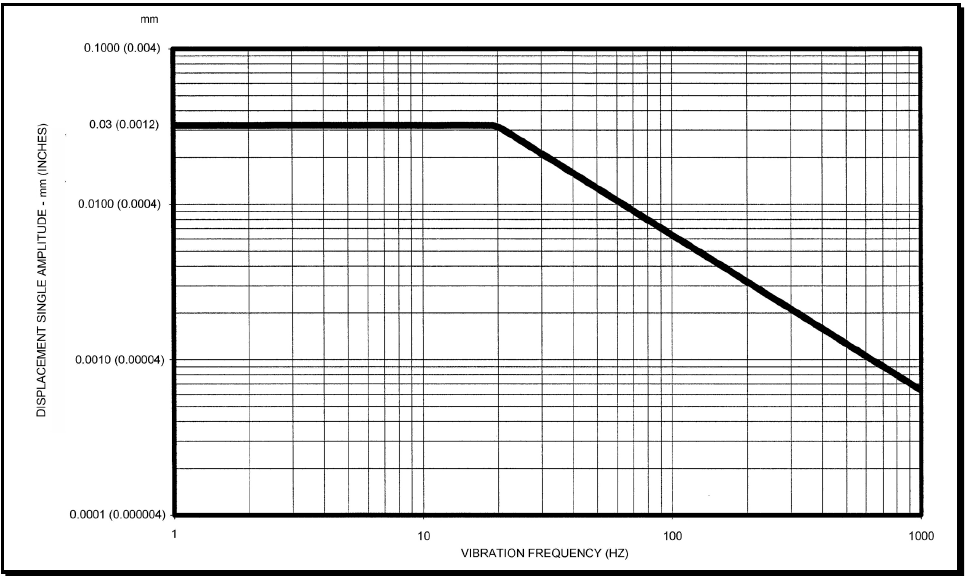
Figure description:
Vibration Displacement Profile Chart
DISPLACEMENT SINGLE AMPLITUDE - mm (INCHES vs. VIBRATION FREQUENCY (HZ
| VIBRATION FREQUENCY (HZ) | DISPLACEMENT SINGLE AMPLITUDE (mm) | DISPLACEMENT SINGLE AMPLITUDE (INCHES) |
|---|---|---|
| 1 | 0.0300 | 0.0012 |
| 10 | 0.0300 | 0.0012 |
| 20 | 0.0300 | 0.0012 |
| 30 | 0.0200 | 0.0008 |
| 40 | 0.0150 | 0.0006 |
| 50 | 0.0120 | 0.00048 |
| 60 | 0.0100 | 0.0004 |
| 100 | 0.0060 | 0.00024 |
| 200 | 0.0030 | 0.00012 |
| 300 | 0.0020 | 0.00008 |
| 400 | 0.0015 | 0.00006 |
| 500 | 0.0012 | 0.000048 |
| 600 | 0.0010 | 0.00004 |
| 800 | 0.00075 | 0.00003 |
| 1000 | 0.0006 | 0.000024 |
Notes: The graph is a log-log plot. It defines a vibration profile with a constant displacement of 0.03 mm from 1 Hz to 20 Hz, and a constant peak velocity region (slope of -1 on log-log displacement vs. frequency from 20 Hz to 1000 Hz.)
Figure 528.1-2. Vibration acceptance criteria for Type II vibration.
5.2.3 Balance Procedure for Flexible Rotors
5.2.3.1 Balance Limits for Flexible Rotors
The residual unbalance for flexible rotors shall not result in vibration displacements larger than specified in Figure 528.1-2 when tested as specified in paragraph 5.2.3.2.
5.2.3.2 Vibration Test Procedure
When mounted as in paragraph 5.2.3.2.1 and measured in accordance with paragraph 5.2.3.2.2, the vibration displacement amplitude at the rotational frequency shall not exceed the values shown on Figure 528.1-2.
5.2.3.2.1 Mounting
The test item shall be completely assembled and mounted elastically at a natural frequency corresponding to less than one-quarter of the frequency associated with the minimal operational speed of the equipment. To accomplish this, the minimum static deflection of the mounting should be determined by Figure 528.1-3, but in no case shall the deflection exceed one-half the original height of the elastic element. On machinery that cannot be mounted as described, the test item shall be mounted on the shipboard mounting for which it is intended, as specified (see Annex B, paragraph 2g(5)).
MIL-STD-810H
METHOD 528.1
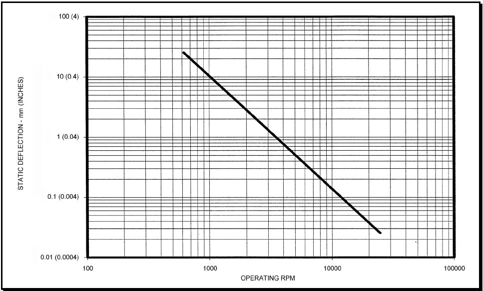
Figure description:
STATIC DEFLECTION vs. OPERATING RPM
| OPERATING RPM | STATIC DEFLECTION - mm | STATIC DEFLECTION - (INCHES) |
|---|---|---|
| 570 | 27.7 | 1.11 |
| 600 | 25.0 | 1.0 |
| 1000 | 9.0 | 0.36 |
| 2000 | 2.25 | 0.09 |
| 3000 | 1.0 | 0.04 |
| 4000 | 0.56 | 0.0225 |
| 5000 | 0.36 | 0.0144 |
| 6000 | 0.25 | 0.01 |
| 8000 | 0.14 | 0.0056 |
| 10000 | 0.09 | 0.0036 |
| 15000 | 0.04 | 0.0016 |
| 20000 | 0.0225 | 0.0009 |
| 25000 | 0.0144 | 0.000576 |
Notes: The chart is a log-log plot showing the relationship between Operating RPM and Static Deflection. The primary units for deflection are millimeters, with equivalent inch measurements provided in parentheses. The y-axis labels indicate a conversion of 25 mm per inch (e.g., 100 mm is labeled as 4 inches. The plotted data follows a power-law relationship approximately defined by Static Deflection (mm = 9,000,000 / (Operating RPM^2.)))
Figure 528.1-3. Minimum static deflection of mounting for Type II vibration test.
5.2.3.2.2 Measurements
Amplitudes of vibration shall be measured on the bearing housing in the direction of maximum amplitude. On constant speed units, measurements shall be made at the operating speed. In the case of variable speed units, measurements shall be made at maximum speed, and at all critical speeds (see paragraph 2.2h) within the operating range. Measurements at many speeds may be required to establish the existence of critical speeds of variable speed units. The maximum frequency step size used when establishing critical speeds shall be 0.25 Hz.
5.2.3.2.3 Instruments
Amplitude and frequency measurements shall be performed with instrumentation that has calibration traceable to the National Institute of Standards and Technology (NIST), and that has dynamic and frequency ranges consistent with the amplitude and frequency range specified in Figure 528.1-2.
5.3 Analysis of Results
In addition to the guidance provided in Part One, paragraph 5.14, the following is provided to assist in the evaluation of the test results.
528.1-5.3 Snow
Three aspects of snow are discussed in relation to materiel design. Falling snow also affects the performance of electro-optical systems because of the attenuation and degradation of electromagnetic radiation in the atmosphere.
- a. Snowfall rate. No operational extreme is given for rate of snowfall accumulation because conditions are more severe when snow is windblown (see paragraph 5.3b below). The greatest snowfall accumulation during a 24-hour period ever recorded in the United States, the snowier sections of which receive as much snow as any part of the world, was 1930 mm (76 inches), a rate of about 76 mm/hr (3 inches per hour). Crystal sizes of snow particles range from 0.05 to 20 mm diameter with a median range of 0.1 to 1.0 mm. Larger sizes are associated with temperatures near freezing and light winds.
- b. Blowing snow. Operational extremes for blowing snow are given in terms of horizontal mass flux of snow particles; that is, the mass of snow moving horizontally across a unit area per unit time. Mass flux decreases significantly with increasing height; highest fluxes are found below 0.05m (2 inches). Therefore, extremes of blowing snow are given for height intervals up to 10m (33 feet). Design values should be based on the height of the materiel. The horizontal mass fluxes for operational extremes, with a wind speed of 13 mps (44 fps) at a height above ground or snow surface of 3m (10 feet), are shown in Table XVIII.
Table XVIII. Horizontal mass fluxes for blowing snow
| Height | Mass Flux | ||
|---|---|---|---|
| feet | meters | lbs./ft/sec | kg/m²/sec |
| 33.0 | 10.0 | 0.45 x 10⁻³ | 2.2 x 10⁻³ |
| 25.0 | 7.5 | 0.68 x 10⁻³ | 3.3 x 10⁻³ |
| 16.0 | 5.0 | 0.82 x 10⁻³ | 4.0 x 10⁻³ |
| 8.2 | 2.5 | 1.4 x 10⁻³ | 6.9 x 10⁻³ |
| 3.3 | 1.0 | 3.3 x 10⁻³ | 16.0 x 10⁻³ |
| 2.5 | 0.75 | 4.5 x 10⁻³ | 22.0 x 10⁻³ |
| 1.6 | 0.5 | 6.6 x 10⁻³ | 32.0 x 10⁻³ |
| 0.82 | 0.25 | 14.0 x 10⁻³ | 66.0 x 10⁻³ |
| 0.33 | 0.1 | 41.0 x 10⁻³ | 200.0 x 10⁻³ |
| 0.16 | 0.05 | 109.0 x 10⁻³ | 530.0 x 10⁻³ |
When blown by strong winds, snow crystals are broken and abraded into roughly equal size grains with rounded or subangular corners. More particles occur in the size range of 0.02mm to 0.4mm, where the size is the effective diameter as in the plane of measurement. Smaller sizes tend to occur at lower temperatures. Within the basic cold regions, the typical temperature range during periods of blowing snow is to to . Within the cold and severe cold regions, snowfall is common at temperatures between and and . Blowing snow may occur at temperatures as low as . Particle size decreases rapidly with height from the surface to 0.05m (1.6 ft), and gradually above this level. A typical distribution of blowing snow particle sizes applicable to extremes is given in the following table.
Table XIX. Typical distribution of blowing snow particle sizes.
| Effective Diameter (micrometers) | |||||||||||||
|---|---|---|---|---|---|---|---|---|---|---|---|---|---|
| 23 | 35 | 47 | 59 | 71 | 83 | 95 | 107 | 119 | 131 | 143 | 155 | 167 | |
| to | to | to | to | to | to | to | to | to | to | to | to | to | |
| 34 | 46 | 58 | 70 | 82 | 94 | 106 | 118 | 130 | 142 | 154 | 166 | 178 | |
| Percent | 0.6 | 1.3 | 5.0 | 15 | 22 | 21 | 16 | 9.7 | 4.7 | 2.5 | 1.0 | 0.7 | 0.5 |
-
c. Snowload. A third important effect of snow is the structural load imposed by accumulated snow upon buildings, shelters, vehicles, or other relatively large military items. Snowload extremes are not applicable to operations; however, designers of the above materiel may wish to consider the following extremes that are for snowloads on the ground. Snowloads on military materiel would usually be less than on the nearby ground.
-
(1) Portable materiel usually involves small items, such as tentege, that may be moved daily. This materiel generally will shed snow, but in instances where it does not, distortion will be noticeable and daily cleaning mandatory. The design criterion for this materiel is based on 24-hour snowfalls. The snowload value is 48.9 kg/m² (10 lbs/ft²), that is equivalent to a depth of 508 mm (20 inches) of snow with a specific gravity of 0.1.
-
(2) Temporary materiel usually involves large items on which snow can collect, rigid shelters, portable hangars, etc., that can be cleared of snow between storms. This materiel will not sag much due to the snow loading, but may collapse when its limits are exceeded. The design criterion for this materiel is based on snowfalls associated with storms lasting longer than one day. The snowload value is 97.7 kg/m² (20 lbs/ft²), is equivalent to a snow depth of 1016 mm (40 inches) with a specific gravity of 0.1.
-
(3) Semi-permanently installed materiel is usually demountable and not very mobile. Snow is not removed between snowfalls. The design criterion for this materiel is based on seasonal accumulation of snow. The snowload value is 235 kg/m² (48 lbs/ft²), that is equivalent to a snow depth of 2438 mm (96 inches) with a specific gravity of 0.1.
-
(a) Highest Recorded. The values given in this section are for snow loads on the ground, not on shelters or materiel. Although snow loads on materiel are generally less than ground snow loads, the latter may be used as a guide in determining the maximum snow loads that are possible. Values, provided as kg/m², can be converted to lbs/ft² by multiplying by 0.205.
-
Portable Materiel. In mountainous areas 194 kg/m²; in non-mountainous areas 137 kg/m². These are based on the extreme 24-hour snowfalls that occurred at Silver Lake, Colorado (193 cm) in April 1921, and Barnes Corner, New York (137 cm) in January 1976, respectively.
-
Temporary Materiel. In mountainous areas, 484 kg/m²; in non-mountainous areas 191 kg/m². These are based on the extreme single-storm snowfalls exceeding 24 hours. They occurred at Mt Shasta, California (480 cm) in February 1959, and Watertown, New York (175 cm) in January 1922, respectively.
-
(b) Semi-permanently Installed Materiel. In mountainous areas, 1155 kg/m²: for non-mountainous areas, the record extreme is not available, but an extreme that is likely to occur one year in 30 is a snow load of 590 kg/m². The estimate for mountainous areas was based on the greatest recorded depth, 1146cm (37.5 ft), that occurred at Tamarack, California in March 1911. The non-mountain value was based on a study of Canadian snowfall statistics.
-
(c) Frequency of Occurrence. Not applicable because materiel should be designed to withstand, without collapse or severe damage, snow loads that are expected over long periods.
-
(d) Long-term Extremes. Snow loads recommended for use in design would be expected to occur one year in ten at the worst non-mountainous areas in the world. They are based on data obtained for stations located in the United States and Canada. The values presented are based on ground snow loads from non-mountainous areas converted to loads on horizontal and exposed surfaces of the materiel over which the wind flow is unimpeded and unobstructed. Inclined surfaces need to support only as much snow as can accumulate on the slope involved.
-
(e) Portable Materiel. 49 kg/m². Based on a 24-hour snowfall to a depth of 51 cm (20 in) with a specific gravity of 0.1.
-
(f) Temporary Materiel. 98 kg/m². Based on a single-storm snow depth of 102 cm (40 in) with a specific gravity of 0.1.
-
(g) Semi-permanently Installed Materiel. 246 kg/m². Based on an estimated ground snowload of 393 kg/m² (80 lb/ft²) one year in 10 (10 percent probability each year), and a conversion factor of 0.625 for determining materiel loads from ground loads.
-
d. Highest Recorded. Highest recorded horizontal mass fluxes (saturation conditions) at heights ranging from 0.05 to 10m, accompanied by a wind speed of 45 knots (52 mph) at the 3m level are:
Table XX. Highest recorded snow mass fluxes.
| Height | Mass Flux | ||
|---|---|---|---|
| (m) | (ft) | (g/m² sec) | (lb/ft² sec) |
| 10 | 33 | 310 | 63x10-3 |
| 7.5 | 25 | 320 | 66 |
| 5.0 | 16 | 330 | 68 |
| 2.5 | 8.2 | 380 | 78 |
| 0.75 | 2.5 | 630 | 129 |
| 0.50 | 1.6 | 800 | 164 |
| 0.25 | 0.82 | 1600 | 328 |
| 0.10 | 0.33 | 3000 | 614 |
| 0.05 | 0.16 | 6200 | 1270 |
- e. Frequency of Occurrence. The horizontal mass fluxes, one percent value, at heights ranging from 0.05 to 10 m, driven by wind speeds of 25 knots (29 mph) at the 3m (10 ft) level (the 1-percent wind speed in central Canada during January) are:
Data for 5- and 10-percent values are not available. Recommend the above values be applied to any material that is susceptible to the effects of blowing snow. The typical particle-size distribution and associated temperature are provided in paragraph 5.3b.
- f. Long-Term Extremes. Not applicable for this climatic element.
5.3.1 Physics of Failure
Analyses of vibration related failures must relate the failure mechanism to the dynamics of the failed item and to the dynamic environment. It is insufficient to determine that something broke due to high cycle fatigue or wear. It is necessary to relate the failure to the dynamic response of the equipment to the dynamic environment. Thus, include in failure analyses a determination of resonant mode shapes, frequencies, damping values and dynamic strain distributions, in addition to the usual equipment properties, crack initiation locations, etc. (See Method 514.8, Annex A, paragraph 2.5, as well as paragraph 6.1, references k and l).
5.3.2 Qualification Tests
When a test is intended to show formal compliance with contract requirements, recommend the following definitions:
- a. Failure definition. "Equipment is deemed to have failed if it suffers permanent deformation or fracture; if any fixed part or assembly loosens; if any moving or movable part of an assembly becomes free or sluggish in operation; if any movable part or control shifts in setting, position or adjustment, and if test item performance does not meet specification requirements while exposed to functional levels and following endurance tests." Crack initiation in a critical structure constitutes failure of the test. Ensure this statement is accompanied by references to appropriate specifications, drawings, and inspection methods.
- b. Test completion. "A vibration qualification test is complete when all elements of the test item have successfully passed a complete test. When a failure occurs, stop the test, analyze the failure and repair the test item. Continue the test until all fixes have been exposed to a complete test. Each individual element is considered qualified when it has successfully passed a complete test. Elements that fail during extended tests are not considered failures, and can be repaired to allow test completion." After testing, check all points of pre-identified stress concentration with a penetrating dye. This dye test will identify areas of crack initiation.
5.3.3 Other Tests
For tests other than qualification tests, prepare success and/or failure criteria and test completion criteria that reflect the purpose of the tests.
5.4 Ice
5.4.1 Icing phenomena
Icing phenomena include glaze (freezing rain), hoarfrost, and rime that cause problems of ice accretion on aircraft and other materiel, and ice fog that interferes with visibility. Although reliable and systematic data on ice accumulation are scarce, fairly large areas of the United States and Europe can expect to endure seven or more ice storms per year. The effects of the storms may last from a few hours to several days. In the same areas, probably one storm per year on the average is severe enough to cause some damage. In perhaps one year out of two or three, ice accumulation will probably be a half-inch or more. Therefore, if all-weather operation of materiel is desired within the areas where icing may occur, the operational design value should be for one-half inch of glaze with specific gravity of 0.9. This includes the colder sections within the basic design type, and all of the cold and severe cold areas. If materiel failure during the time of icing can be tolerated, the question of withstanding more severe storms without permanent damage becomes important. For withstanding, the values are as follows:
76 mm (3 inches) glaze, specific gravity 0.9.
- 152 mm (6 inches) glaze and rime mixed, specific gravity 0.5.
152 mm (6 inches) rime, specific gravity 0.6.
152 mm (6 inches) rime near the surface increasing linearly to 508mm (20 inches) at
122m (400 feet), specific gravity 0.2.
- a. Deposits of hoarfrost, the only type of ice accretion that occurs when air temperatures are well below 0°C (32°F), may be several inches thick but will have a specific gravity of less than 0.2.
- b. Ice fog consists of suspended ice crystals averaging 5 to 20 micrometers in diameter. In areas where sufficient water vapor is present, ice fog occurs mainly at temperatures below -37°C (-35°F). Ice fog may be very dense, limiting visibility to a few feet. This condition is often locally induced by the operation of motor vehicles, power plants, weapon systems. It is usually high in concentration of contaminants from
MIL-STD-810H
PART THREE
the burning of hydrocarbon fuels and explosive fuels. It affects the performance of electro-optical systems because of its attenuation and degradation of electromagnetic radiation in the atmosphere.
5.4.2 Ice accretion
Ice accretion can be a major destructive force to structures, such as towers, located in middle and high latitudes just about anywhere in the world. Concurrent or subsequent strong winds may be the critical force in damaging materiel loaded with ice. There are three basic kinds of ice formed by accretion in the atmosphere: glaze, hard rime, and soft rime.
Glaze occurs when rain (sometimes drizzle) freezes on objects; it is clear and nearly as dense as pure ice. Hard rime is less transparent than glaze because of air trapped in the ice. The density with respect to water (specific gravity) varies from 0.6 to 0.9. It is usually the result of freezing drizzle, but may occur from exposure to supercooled cloud droplets during high winds with the temperature near freezing. Soft rime ice occurs when supercooled clouds or fog droplets freeze upon impact with surfaces colder than 0°C (32°F). It is opaque with a specific gravity of 0.2 to 0.5. It occurs most commonly on hills or mountaintops exposed to clouds at freezing temperatures.
Unfortunately, quantitative records of glaze and rime are not available because icing has not been routinely observed at operational weather stations. In order to determine reasonable values of ice and wind loading, it was necessary to study case histories of major ice storms, when structures have failed due to the strain of combined ice and wind loading.
- a. Highest Recorded. Not available.
- b. Frequency of Occurrence. Except for locations such as mountaintops exposed to supercooled clouds, the frequency of occurrence is normally quite low. Materiel exposed to the environment should be designed to survive the extreme accumulation of ice and concurrent wind expected to occur once over a period of years.
- c. Long-Term Extremes. These values are estimated to occur once in ten years at icing-prone locations such as eastern Labrador, Canada. More severe conditions will be found on cloud-immersed mountain peaks during periods of continuous passage of supercooled water clouds (specific information will be required for materiel designed especially for such installations). Strong winds are frequently associated with icing, occurring during its formation or after it has formed but before melting. Forces of such winds must be added to forces due to ice accretion as part of the stress in design for ice accretion.
Values of ice provided in paragraph 5.4.1 above are thicknesses extending horizontally into the wind. They apply to structures extending up to heights of 125m (410 ft). Associated wind loading can be considered as gusts of 100 knots (115 mph) at about 10m (33 ft), increasing to 123 knots (142 mph) at 125m (410 ft/min). Use independent design considerations for the value of each of the three types of icing below:
5.5 Atmospheric pressure. Atmospheric pressure usually is not considered in the design and testing of military materiel. Ambient pressure, however, may be important for a few types of materiel, for example, items that require oxygen for combustion and sealed units, that might explode or collapse under abnormally low or high pressure.
- a. High pressure. The operational extreme high pressure is 108 kPa (31.89 inches).
- b. Low pressure. The operational extreme low pressure is estimated to be 50.8 kPa (15.00 inches) at 4,572m (15,000 feet), the highest elevation at which Army materiel is likely to be used. At sea level, the operational extreme is 87.7 kPa (25.90 inches).
5.6 Ozone concentration
See MIL-HDBK-310, paragraph 5.1.20.
5.7 Sand and dust
“Sand” and “dust” are terms used to designate small particles of matter, usually of mineral origin. A distinction is often made between sand and dust on the basis of size, but there are no generally accepted specific size limits for the two kinds of particles. For most military applications, it is important to distinguish between the smaller particles (dust) and the larger particles (sand) because of their primary effects on materiel. Airborne dust is primarily damaging because of its penetration and subsequent possible damage; airborne sand is primarily damaging because of its erosion and abrasion effects on materiel. Particles vary in diameter from 0.1 to 1,000 micrometers (3.94 x 10⁻⁶ inches to 3.94 x 10⁻² inches), but most airborne particles are less than 74 micrometers (2.91 x 10⁻³ inches). Dust can penetrate small openings, causing undue wear to moving parts, and interfere with electrical contacts. Hardness also varies widely (from 1 to 9 on the Mohs scale) depending largely on mineral composition. Blowing sand, that may be too large to penetrate the smaller openings, can erode and abrade the outside of materiel. Sand and dust present in the air affect
MIL-STD-810H
PART THREE
the performance of electro-optical systems because of their attenuation and degradation of electromagnetic radiation in the atmosphere. Greatest particle concentrations are found near helicopters hovering over dry, loose surfaces. Secondary concentrations are found near ground vehicles operating on unpaved surfaces. Lesser concentrations are associated with natural dust storms, although the areal extent of such storms may be substantial.
- a. Highest Recorded. Too few reliable and systematic measurements have been made to establish an extreme value. However, concentrations as high as 6.00 g/m² (particles smaller than 70 micrometers) have been made inside the engine compartment of a tank moving over a very dusty surface.
- b. Frequency of Occurrence. Since this is not an observed climatic element, and is most often mechanically created, frequencies of occurrence are not applicable. Three concentration levels are provided; selection of the appropriate one depends on intended use of the materiel under consideration. Items likely to be used in close proximity to aircraft operating over unpaved surfaces should be designed for particle concentrations of about 2.19 g/m3 in multidirectional strong winds (downwash from helicopters rotors). Such particles range in size up to 500 µm in diameter. Items never used in close proximity to operating aircraft, but which may be found near operating surface vehicles, should be designed for particle concentrations of 1.06 g/m3 with wind speeds up to 18 mps at a height of 3m. Particle sizes will range from less than 74 µm in diameter to 1000µm, with the bulk of the particles ranging in size between 74 and 350µm. These two categories are likely to include most military items. However, items that are assured of being subjected to ONLY natural conditions should be designed for particle concentrations of 0.177 g/m3 with wind speeds of 18 m/s at a height of 3m (10 ft). Under these conditions, the bulk of the particle sizes are likely to be less than 150 µm, except that some larger particles (up to 1000 µm) may be in motion within several feet above the ground. In all categories, temperatures are typically above 21oC (70oF) and relative humidities are less than 30 percent. For testing purposes, particle sizes up to 150 µm should be used if the primary concern is with the penetration of fine particles. If the abrasion effect of blowing sand is the primary concern, particle sizes up to 1000 µm should be used, but the bulk of the particles should be between 150 and 500 µm. Many items, such as rifles, vehicles, and helicopters, may be exposed to fine particles that can penetrate the space between moving parts.
5.8 Dust as a natural obscurant
Airborne dust scatters visible, near-IR, and thermal radiation. The scattering shows little spectral sensitivity in the visible and near-IR bands because of the relatively broad particle size distribution. Transmittance losses in the thermal bands are slightly lower than in the visible region and may show some spectral dependence.
Airborne dust and sand may be either part of a constant background aerosol or a dust cloud that may persist in duration from less than an hour to several days. Dust storms (visibility < 1 km due to dust) are common phenomena over many parts of the world, and in some areas they occur with great frequency (see Table XXI). The dust fall from these storms has been estimated to extend over as much as 575,000 to 800,000 km². Major regions where dust originates are the Sahara, the southern coast of the Mediterranean Sea, the northeast Sudan, the Arabian Peninsula, the lower Volga and North Caucasus in the former USSR, the pampas of Argentina, Afghanistan, and the western Great Plains of the US.
Worldwide dust storm frequency is at a maximum in areas where the annual rainfall is between 100 and 200 mm (3.9 and 7.9 in); in such locations the mean annual frequency is about nine days per year.
MIL-STD-810H
PART THREE
Table XXI. Number of days per year with dust storms (visibility < 1 km)
| Location | Days Per Year |
|---|---|
| Abadan, Iran | 13 |
| New Delhi, India | 8 |
| Ganganagar, India | 17 |
| Paoting, China | 19 |
| Kantse, China | 35 |
| Hami, China | 33 |
| Tarim Basin, China | 100 to 174 |
| Baghdad, Iraq | 21 |
| Basra, Iraq | 15 |
| Shaibah, Iraq | 38 |
| Diwaniyah, Iraq | 36 |
| Aqaba, Jordan | 11 |
| Nguru, Nigeria | 26 |
| Mexico City, Mexico | 68 |
| Kazakhstan, (former) USSR | 60 |
| Repetek, (former) USSR | 60 |
| Beersheva, Israel | 27 |
| Kuwait Airport, Kuwait | 27 |
| Abu Kamal, Syria | 10 |
| Mersa Matruh, Egypt | 10 |
| Riyadh, Saudi Arabia | 13 |
| Dharan, Saudi Arabia | 11 |
| Khartoum, Sudan | 24 |
Size distributions of dust usually fall into three categories. The first category, between 1 and 10 μm in radius, appears to be characteristic of soil-derived aerosols under all conditions. This distribution is generally present and is not related to the size distribution of soil over which measurements are taken. The second category, occurring between 10 and 100 μm, appears to be characteristic of the parent soil size distribution only under conditions of moderate-to-heavy dust loading in the atmosphere. The third category, centered between 0.02 and 0.5 μm, generally does not appear related to the other (soil) modes in composition or origin; rather, it appears to be characteristic of a background aerosol and may be identified with the accumulation mode for secondary aerosols observed in urban measurements.
MIL-STD-810H
PART THREE
5.9 Freeze-thaw cycles
A freeze-thaw cycle occurs at a specific site on any day the temperature crosses the freezing mark. It is possible for more than one freeze-thaw cycle to occur at any site during a 24-hour period, however, because of normal control of the daily temperature cycle by the solar cycle, this is not a common occurrence. Therefore, freeze-thaw cycles are described by the number of days in which they occur.
- a. Freeze-thaw is an important consideration in the design of many types of military materiel. Consider it in the design of all materiel to be used in the areas where freeze-thaw cycles occur. The effects on materiel are caused by alternating expansion and contraction of different materials and, especially, the change of state that water experiences during the freezing and thawing processes. The freezing and thawing of water in exposed components of materiel can create great internal stress and damage. Freeze-thaw is of greatest potential concern as a factor affecting materiel in areas where abundant moisture is present (so that condensation and precipitation are common) immediately before or during the occurrence of the freeze-thaw cycle. The maximum number of freeze-thaw days in non-mountainous areas occurs in the mid-latitudes. The mid-latitudes also have a great variance in average number of freeze-thaw days. In general, sites that have the most months with mean monthly temperatures at or near 0°C (32°F) will have the greatest annual number of freeze-thaw days in non-mountainous areas. However, materiel should be designed to withstand at least 20 cycles during the most severe month, with concurrent dewpoints of -2°C to 2 C (28°F to 36°F), a trace or more precipitation on the day of the cycle, and humidities tending toward saturation.
- b. In tropical mountains at high elevations, freeze-thaw cycles 337 days annually, and 31 days per month have been recorded. Elsewhere, a maximum of 31 days in one month also have been recorded.
- c. Due to the nature of this climatic condition, frequency of occurrence expressed as a percent does not apply. An occurrence of 20 cycles during the worst month is recommended. This would occur in low-level, mid-latitude areas such as Germany.
- d. Operational values are not appropriate for this element. However, materiel should be designed to withstand at least 20 cycles during the most severe month, with concurrent dewpoints of -2°C to 2 C (28°F to 36°F), a trace or more precipitation on the day of the cycle, and humidities tending toward saturation.
5.9.1 Basic cold-wet cycle
Note: Although details for the cold-wet cycle are not included, the following general information provides guidance. This cycle was developed by the Corps of Engineers, but was never adopted by the US Army.
Basic cold-wet conditions occur throughout the colder, humid sections of the basic (regional) design type adjoining the areas of basic cold conditions. Cold-wet conditions, as defined here, may occur in any part of the basic type that regularly experiences freezing and thawing on a given day; however the conditions are found most frequently in Western Europe, the central United States, and northeastern Asia (China and Japan). In the Southern Hemisphere, cold-wet conditions occur only at moderately high elevations except in South America where they are found in Argentina and Chile south of 40° latitude.
Table XXII. Cold-wet daily cycle of temperature, humidity, and solar radiation.
| Local Time | OPERATIONAL CONDITIONS (Natural Environment) | STORAGE AND TRANSIT CONDITIONS | ||||||||
|---|---|---|---|---|---|---|---|---|---|---|
| Ambient Air Temperature | Solar Radiation | Relative Humidity | Dewpoint Temperature | Induced Air Temperature | Relative Humidity | |||||
| °C | °F | W/m² | Bph | Percent | °C | °F | °C | °F | Percent | |
| 0100 | -3 | 26 | Negligible During Low Temperature Periods | Tending Towards Saturation | -3 | 26 | -4 | 25 | Tending Toward Saturation | |
| 0200 | -3 | 26 | -3 | 26 | -4 | 24 | ||||
| 0300 | -4 | 25 | -4 | 25 | -5 | 23 | ||||
| 0400 | -4 | 25 | -4 | 25 | -5 | 23 | ||||
| 0500 | -4 | 25 | -4 | 25 | -5 | 23 | ||||
| 0600 | -4 | 25 | -4 | 25 | -5 | 23 | ||||
| 0700 | -3 | 26 | -3 | 26 | -4 | 24 | ||||
| 0800 | -2 | 28 | -2 | 28 | -3 | 26 | ||||
| 0900 | -1 | 30 | -1 | 30 | -1 | 29 | ||||
| 1000 | 0 | 32 | 0 | 32 | 0 | 32 | ||||
| 1100 | 1 | 33 | 1 | 33 | 1 | 34 | ||||
| 1200 | 1 | 34 | 1 | 33 | 2 | 36 | ||||
| 1300 | 2 | 35 | 1 | 34 | 3 | 37 | ||||
| 1400 | 2 | 35 | 1 | 34 | 3 | 37 | ||||
| 1500 | 2 | 35 | 1 | 34 | 3 | 37 | ||||
| 1600 | 1 | 34 | 1 | 33 | 2 | 36 | ||||
| 1700 | 1 | 33 | 1 | 33 | 1 | 34 | ||||
| 1800 | 0 | 32 | 0 | 32 | 1 | 33 | ||||
| 1900 | -1 | 30 | -1 | 30 | 0 | 32 | ||||
| 2000 | -2 | 29 | -2 | 29 | -1 | 30 | ||||
| 2100 | -2 | 28 | -2 | 28 | -2 | 29 | ||||
| 2200 | -3 | 27 | -3 | 27 | -2 | 28 | ||||
| 2300 | -3 | 27 | -3 | 27 | -3 | 27 | ||||
| 2400 | -3 | 26 | -3 | 26 | -3 | 26 | ||||
5.10 Microbial growth (fungus / mould)
Method 508.6 includes a list of fungus species typically used for US applications.
Although not specifically an “environmental element,” and as previously stated (paragraph 2.2.2), microbial deterioration is a function of temperature and humidity and is an inseparable condition of hot humid tropics and the mid-latitudes. Consider microbial deterioration in the design of all standard general-purpose materiel. NATO documentation provides an additional list as shown in Table XXIII below.
MIL-STD-810H
PART THREE
Table XXIII. European test fungus species.
| Fungus | Fungus Sources Identification No. | Materials affected | |
|---|---|---|---|
| USDA1 | ATCC2/ | ||
| Aspergillus niger | QM 458 | ATCC 6275 | Textiles, vinyl, conformal coatings, insulation, adhesives, etc. Resistant to tanning salts and copper |
| Aspergillus terreus | QM 82j | ATCC 10690 | Haversack, paperboard, paper, plastics |
| Paecilomyces variotii | QM 6764 | IAM 50013/ATCC 18502 | Plastics, leather, textiles |
| Penicillium funiculosum | ATCC 36839 IAM 70134/ | Textiles, plastics, cotton fabric, polymers, automotive components such as gaskets, distributors, cables, hoses, PVC, airborne equipment such as breakers, solenoids, switches, remote transmission accessories | |
| Penicillium ochro-chloron | QM 477 | ATCC 9112 | Plastics, textiles |
| Scopulariopsis brevicaulis | ATCC 36840 | Rubber | |
| Trichoderma virens (ATCC 9645) | QM 365 | ATCC 9645 | Plastics, textiles, packing materials |
| (Gliocladium virens IAM 5061) | IAM 50614/ | ||
5.11 Hail
Hail occurs too infrequently to warrant specification of an operational extreme. When hail-caused materiel failure would endanger life or limb, designers should consider the possibility of encountering hailstones up to 51 mm (2 inches) in diameter. The largest hailstone ever recorded measured 47.6 cm (18.75 inches) in diameter (see Annex A, Table A-II).
5.12 Combined environmental effects
The climatic design types in this Section are based primarily on temperature extremes, and secondly on humidity extremes. The climatic elements discussed in paragraph 3.5, however, may interact concurrently with temperature and humidity and with each other to produce effects on materiel either different or more severe than the sum of the effects caused by the separate elements acting independently. These are known as combined or synergistic environmental effects. The fact that these synergistic effects exist is one of the prime arguments for conducting field tests, because it is extremely difficult or impossible to reproduce the interacting environmental factors concurrently in a test chamber.
5.13 High elevations and upper air conditions
- a. For materiel subject to transport through high mountain passes, the temperatures and pressures for elevations as high as 4,572 meters (15,000 feet) apply.
- b. For materiel subject to shipment by air (elevations as high as 15,240 meters or 50,000 feet), the low air pressure and temperature shown below could result from failure of cabin pressure and temperature regulation.
Table XXIV. Low air pressure and temperature at elevation.
| Height or Elevation | Pressure | Temperature | ||
|---|---|---|---|---|
| Meters | Feet | Kilopascals (kPa) | °C | °F |
| 3048 | 10,000 | 66 | -41 | -42 |
| 4572 | 15,000 | 52 | -47 | -53 |
| 6096 | 20,000 | 41 | -56 | -68 |
| 9144 | 30,000 | 25.5 | -66 | -87 |
| 12192 | 40,000 | 16 | -72 | -98 |
| 15240 | 50,000 | 10 | -76 | -105 |