516.8-2 COMPLEX SHOCKS
This Method and this Annex are focused upon simple shocks such as in Figure 516.8-A1 (and repeated below as Figure 516.8B-1). Many shocks are not simple in nature. Figure 516.8B-2 displays a complex shock. The phenomenon producing this shock would appear to have three “rebounds.” If it can be traced to a distinct phenomenon, the last of the four shocks might be separated out as a simple shock from the other three. A trained analyst and a clear understanding of the shock producing phenomenon are needed to justify any such decomposition of this complex shock. It probably would not be possible to use SRS synthesis for laboratory test, leaving TWR as the only option for laboratory testing. Cases in which it would appear that several “simple shocks” are in series should rely upon a trained analyst to identify individual “simple shocks” in concert with goals of the characterization, analysis, and specification. Any decomposition of a series of shocks should be related to the phenomenon producing the shock. For example, a catapult shock represents a non-simple shock that could be specified as two independent simple shocks, separated in time by approximately three seconds with an intervening transient vibration. See Figure 516.8-11. Gunfire Shock, Method 519.8, presents information on a repeated shock, the repetition rate being the gun-firing rate. The direct replication method is preferred over the synthesis method when non-simple shocks are being considered.
Generally, this Method has no recommendations beyond the use of TWR for laboratory test specification and laboratory testing for such complex shocks. It is important to maintain the integrity of the complex shock to the extent possible.
MIL-STD-810H METHOD 516.8 ANNEX B
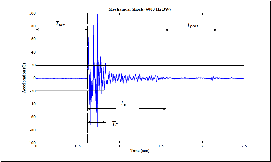
Figure description:
Mechanical Shock (6000 Hz BW Acceleration vs Time Trace
Mechanical Shock (6000 Hz BW
Annotations
- T_pre (text_label - position: x from 0 to 0.62)
- T_post (text_label - position: x from 1.56 to 2.18)
- T_E (text_label - position: x from 0.62 to 0.83)
- T_e (text_label - position: x from 0.62 to 1.56)
- Shock Start (vertical_line - position: x = 0.62)
- Shock Intensity End (vertical_line - position: x = 0.83)
- Shock Event End (vertical_line - position: x = 1.56)
- Post-shock End (vertical_line - position: x = 2.18)
- Zero acceleration baseline (horizontal_line - position: y = 0)
| Time (sec) | Acceleration (G) |
|---|---|
| 0.00 | 0.2 |
| 0.20 | -0.1 |
| 0.40 | 0.3 |
| 0.60 | -0.2 |
| 0.62 | 0.0 |
| 0.63 | 64.0 |
| 0.64 | -42.0 |
| 0.65 | 45.0 |
| 0.66 | -55.0 |
| 0.67 | 82.0 |
| 0.68 | -48.0 |
| 0.69 | 30.0 |
| 0.70 | -68.0 |
| 0.71 | 25.0 |
| 0.72 | 98.5 |
| 0.73 | -40.0 |
| 0.74 | 20.0 |
| 0.75 | -76.0 |
| 0.77 | 56.0 |
| 0.79 | -22.0 |
| 0.81 | 32.0 |
| 0.83 | 12.0 |
| 0.90 | 14.0 |
| 0.95 | -12.0 |
| 1.00 | 10.0 |
| 1.10 | -8.0 |
| 1.20 | 7.0 |
| 1.35 | -6.0 |
| 1.50 | 4.0 |
| 1.56 | 0.0 |
| 1.70 | -1.0 |
| 1.90 | 0.5 |
| 2.10 | 4.5 |
| 2.18 | -2.0 |
| 2.30 | 0.2 |
| 2.50 | 0.0 |
Notes: The graph depicts a high-frequency mechanical shock measurement. T_pre and T_post represent ambient background periods before and after the event. T_E identifies the duration of the peak impulse, while T_e encompasses the full duration of the transient event including structural ringing/decay.
Figure 516.8B-1. Shock time history with segment identification and O̟ and Т time intervals illustrated.
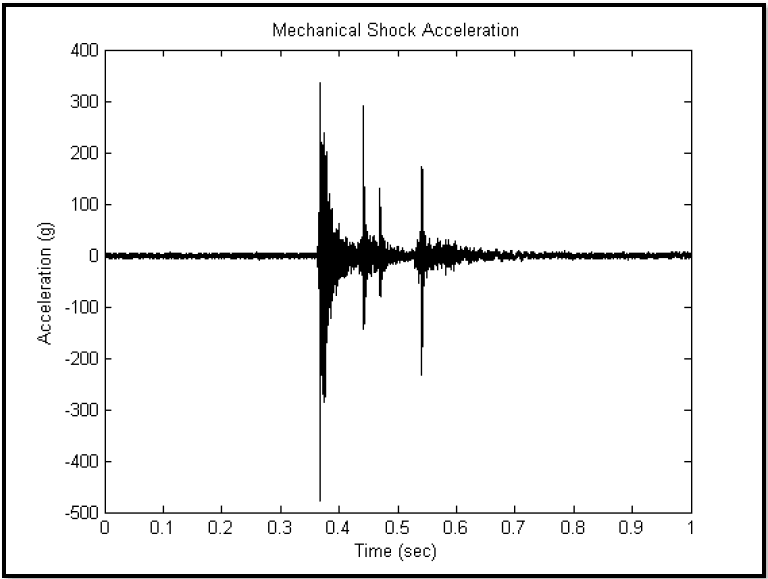
Figure description:
Mechanical Shock Acceleration
Mechanical Shock Acceleration
| Time (sec) | Acceleration (g) |
|---|---|
| 0.0 | 0 |
| 0.1 | 3 |
| 0.2 | -4 |
| 0.3 | 2 |
| 0.36 | -10 |
| 0.365 | -480 |
| 0.37 | 340 |
| 0.375 | -280 |
| 0.38 | 230 |
| 0.4 | 40 |
| 0.43 | -140 |
| 0.44 | 295 |
| 0.45 | 50 |
| 0.47 | 135 |
| 0.5 | 130 |
| 0.54 | 175 |
| 0.545 | -230 |
| 0.6 | 30 |
| 0.7 | 10 |
| 0.8 | -5 |
| 0.9 | 4 |
| 1.0 | 0 |
Notes: The chart shows a high-frequency acceleration signal with three major transient events (shocks occurring between 0.35 and 0.6 seconds. The maximum negative peak is approximately -480g and the maximum positive peak is approximately 340g.)
Figure 516.8B-2. A complex shock.
MIL-STD-810H
METHOD 516.8 ANNEX B
516.8-2 DEVELOPMENT
2.1 Selecting the Shock Method
After examining requirements documents and applying the tailoring process in Part One of this Standard to determine where mechanical shock environments are foreseen in the life cycle of the materiel, use the following to confirm the need for this Method and to place it in sequence with other methods.
516.8-2.1 Limit Estimate Set Selection
It is assumed that the analyst has clearly defined the objective of the prediction and/or measurement assessment, i.e., to provide a statistically viable limit estimate. Prediction estimates, measurement estimates, or a combination of prediction and measurement estimates may be considered in the same manner. It is assumed that uncertainty in individual measurements (processing error) does not affect the limit considerations. For measured field data digitally processed such that estimates of the ASD, SRS, ESD, or FS are obtained for single sample records, it is imperative to summarize the overall statistics of "similar" estimates selected in a way so as to not bias the limits. Since excessive estimate variance at any independent variable value may lead to overly conservative or meaningless limits depending upon the procedure selected, this choice of “similar estimates” is a way of controlling the variance in the final limit estimates. To ensure that similar estimates are not physically biased, the measurement locations might be chosen randomly, consistent with the measurement objectives. Likewise, similar estimates may be defined as (1) estimates at a single location on materiel that has been obtained from repeated testing under essentially identical experimental conditions; (2) estimates on materiel that have been obtained from one test, where the estimates are taken (a) at several neighboring locations displaying a degree of response homogeneity, or (b) in "materiel zones," i.e., points of similar response at varying locations, or (3) some combination of (1) and (2). In any case, similar estimates assume that there is a certain degree of homogeneity among the estimates across the frequency band of interest.
2.1.1 Effects of Shock
Mechanical shock has the potential for producing adverse effects on the physical and functional integrity of all materiel. In general, the damage potential is a function of the amplitude, velocity, and the duration of the shock. Shocks with frequency content that correspond with materiel natural frequencies will magnify the adverse effects on the materiel's overall physical and functional integrity.
The materiel response to the mechanical shock environment will, in general, be highly oscillatory, of short duration, and have a substantial initial rise time with large positive and negative peak amplitudes of about the same order of magnitude (for high velocity impact shock, e.g., penetration shocks, there may be significantly less or no oscillatory behavior with substantial area under the acceleration response curve). The peak responses of materiel to mechanical shock will, in general, be enveloped by a decreasing form of exponential function in time. In general, mechanical shock applied to a complex multi-modal materiel system will cause the materiel to respond to (1) forced frequencies of a transient nature imposed on the materiel from the external excitation environment, and (2) the materiel's resonant natural frequencies either during or after application of the external excitation environment. Such response may cause:
- a. Materiel failure as a result of increased or decreased friction between parts, or general interference between parts.
- b. Changes in materiel dielectric strength, loss of insulation resistance, variations in magnetic and electrostatic field strength.
- c. Materiel electronic circuit card malfunction, electronic circuit card damage, and electronic connector failure. (On occasion, circuit card contaminants having the potential to cause short circuit may be dislodged under materiel response to shock.)
- d. Permanent mechanical deformation of the materiel as a result of overstress of materiel structural and non- structural members.
- e. Collapse of mechanical elements of the materiel as a result of the ultimate strength of the component being exceeded.
- f. Accelerated fatiguing of materials (low cycle fatigue).
- g. Potential piezoelectric activity of materials.
- h. Materiel failure as a result of cracks in fracturing crystals, ceramics, epoxies, or glass envelopes.
2.1.2 Sequence Among Other Methods
- a. General. Use the anticipated life cycle sequence of events as a general sequence guide (see Part One, paragraph 5.5).
MIL-STD-810H
METHOD 516.8
- b. Unique to this Method. Sequencing among other methods will depend upon the type of testing, i.e., developmental, qualification, endurance, etc., and the general availability of test items for test. Normally, schedule shock tests early in the test sequence, but after any vibration tests with the following additional guidelines:
- (1) If the shock environment is deemed particularly severe, and the chances of materiel survival without structural or operational failure are small, the shock test should be first in the test sequence. This provides the opportunity to redesign the materiel to meet the shock requirement before testing to the more benign environments.
- (2) If the shock environment is deemed severe, but the chance of the materiel survival without structural or functional failure is good, perform the shock test after vibration and thermal tests, allowing the stressing of the test item prior to shock testing to uncover combined mechanical and thermal failures.
- (3) There are often advantages to applying shock tests before climatic tests, provided this sequence represents realistic service conditions. Test experience has shown that climate-sensitive defects often show up more clearly after the application of shock environments. However, internal or external thermal stresses may permanently weaken materiel resistance to vibration and shock that may go undetected if shock tests are applied before climatic tests.
2.2 Selecting a Procedure
Table 516.8-I summarizes the eight test procedures covered in the Method with respect to the applicable configurations and operation states of the unit under test.
| Procedure | Description | Packaged | Unpackaged | Operational | Non- Operational |
|---|---|---|---|---|---|
| I | Functional Shock | X | X | ||
| II | Transportation Shock | X | X | X | |
| III | Fragility | X | X | ||
| IV | Transit Drop | X | X | X | |
| V | Crash Hazard Shock | X | |||
| VI | Bench Handling | X | X | ||
| VII | Pendulum Impact | X | X | ||
| VIII | Catapult Launch/Arrested Landing | X | X | X |
516.8-2.2 Estimate Processing Considerations
Once the set of “similar estimates” has been identified the following list of assumptions can be used to ensure limit determination is meaningful.
- a. All estimates are defined over the same bandwidth and at the same independent variable (this is referred to as a “fixed design”).
MIL-STD-810H METHOD
2.2.1 Procedure Selection Considerations
Based on the test data requirements, determine which test procedure, combination of procedures, or sequence of procedures is applicable. In many cases, one or more of the procedures will apply. Consider all shock environments anticipated for the materiel during its life cycle, both in its logistic and operational modes. When selecting procedures, consider:
- a. The Operational Purpose of the Materiel. From requirement documents, determine the operations or functions to be performed by the materiel before, during and after the shock environment.
- b. The Natural Exposure Circumstances. Procedures I through VII are based on single shock events that result from momentum exchange between materiel or materiel support structures and another body. Procedure VIII (Catapult Launch/Arrested Landing) contains a sequence of two shocks separated by a comparatively short duration transient vibration for catapult launch, and a single shock for arrested landing.
MIL-STD-810H
METHOD 516.8
- c. Data Required. The test data required to document the test environment, and to verify the performance of the materiel before, during, and after test.
2.2.2 Difference Among Procedures
- a. Procedure I - Functional Shock. Procedure I is intended to test materiel (including mechanical, electrical, hydraulic, and electronic) in its functional mode, and to assess the physical integrity, continuity, and functionality of the materiel to shock. In general, the materiel is required to function during and after the shock, and to survive without damage resulting from shocks representative of those that may be encountered during operational service.
- b. Procedure II - Transportation Shock. Procedure II is used to evaluate the response of an item or restraint system to transportation environments that create a repetitive shock load. The procedure uses a classical terminal peak sawtooth, either measured or a synthetic shock waveform, to represent the shock excitation portion of the transportation scenario. The shock can be a repetitive event of similar amplitude, or an irregular event that varies in amplitude and frequency bandwidth. Ground vehicle transportation is a common source for transportation shock. Procedure II is not equivalent or a substitute for Method 514.8, Secured Cargo Vibration or Category 5, Loose Cargo, or other Method 516.8 shock test procedures.
- c. Procedure III - Fragility. Procedure III is used early in the item development program to determine the materiel's fragility level, in order that packaging, stowage, or mounting configurations may be designed to protect the materiel's physical and functional integrity. This procedure is used to determine the critical shock conditions at which there is chance of structural and/or operational system degradation based upon a systematic increase in shock input magnitudes. To achieve the most realistic criteria, perform the procedure at environmental temperature extremes.
- d. Procedure IV - Transit Drop. Procedure IV is a physical drop test, and is intended for materiel either outside of, or within its transit or combination case, or as prepared for field use (carried to a combat situation by man, truck, rail, etc.). This procedure is used to determine if the materiel is capable of withstanding the shocks normally induced by loading and unloading when it is (1) outside of its transit or combination case, e.g., during routine maintenance, when being removed from a rack, being placed in its transit case, etc., or (2) inside its transit or combination case. Such shocks are accidental, but may impair the functioning of the materiel. This procedure is not intended for shocks encountered in a normal logistic environment as experienced by materiel inside bulk cargo shipping containers (ISO, CONEX, etc.). See Procedure II (Transportation Shock), and Procedure VII (Pendulum Impact).
- e. Procedure V - Crash Hazard Shock Test. Procedure V is for materiel mounted in air or ground vehicles that could break loose from its mounts, tiedowns, or containment configuration during a crash, and present a hazard to vehicle occupants and bystanders. This procedure is intended to verify the structural integrity of materiel mounts, tiedowns or containment configuration during simulated crash conditions. Use this test to verify the overall structural integrity of the materiel, i.e., parts of the materiel are not ejected during the shock. In some instances, the crash hazard can be evaluated by a static acceleration test (Method 513.8, Procedure III, or a transient shock (Method 516.8, Procedure V)). The requirement for one or both procedures must be evaluated based on the test item.
- f. Procedure VI - Bench Handling. Procedure VI is intended for materiel that may typically experience bench handling, bench maintenance, or packaging. It is used to determine the ability of the materiel to withstand representative levels of shock encountered during such environments. This procedure is appropriate for materiel out of its transit or combination case. Such shocks might occur during materiel repair. This procedure may include testing for materiel with protrusions that may be easily damaged without regard to gross shock on the total materiel. The nature of such testing must be performed on a case-by-case basis, noting the configuration of the materiel protrusions, and the case scenarios for damage during such activities as bench handling, maintenance, and packaging.
- g. Procedure VII – Pendulum Impact. Procedure VII is intended to test the ability of large shipping containers to resist horizontal impacts, and to determine the ability of the packaging and packing methods to provide protection to the contents when the container is impacted. This test is meant to simulate accidental handling impacts, and is used only on containers that are susceptible to accidental end impacts. The pendulum impact test is designed specifically for large and/or heavy shipping containers that are likely to be handled mechanically rather than manually.
MIL-STD-810H
METHOD 516.8
NOTE: The rail impact test, formerly Procedure VII, has been moved to Method 526.2.
- h. Procedure VIII - Catapult Launch/Arrested Landing. Procedure VIII is intended for materiel mounted in or on fixed-wing aircraft that is subject to catapult launches and arrested landings. For catapult launch, materiel may experience a combination of an initial shock followed by a low level transient vibration of some duration having frequency components in the vicinity of the mounting platform’s lowest frequencies, and concluded by a final shock according to the catapult event sequence. For arrested landing, materiel may experience an initial shock followed by a low level transient vibration of some duration having frequency components in the vicinity of the mounting platform’s lowest frequencies.
2.3 Determine Test Levels and Conditions
Having selected this Method and relevant procedures (based on the materiel's requirements documents and the tailoring process), complete the tailoring process by identifying appropriate parameter levels, applicable test conditions, and test techniques for the selected procedures. Base these selections on the requirements documents, the Life Cycle Environmental Profile (LCEP), and information provided with the appropriate procedure. Many laboratory shock tests are conducted under standard ambient test conditions as discussed in Part One, paragraph 5. However, when the life cycle events being simulated occur in environmental conditions significantly different than standard ambient conditions, consider applying those environmental factors during shock testing. Individual climatic test procedures of this Standard include guidance for determining levels of other environmental loads. For temperature- conditioned environmental tests, (high temperature tests of explosive or energetic materials in particular), consider the materiel degradation due to extreme climatic exposure to ensure the total test program climatic exposure does not exceed the life of the materiel. (See Part One, paragraph 5.19.). Consider the following when selecting test levels:
516.8-2.3 Parametric Upper Limit Statistical Estimate Assumptions
In all the formulas for the estimate of the statistical upper limit of a set of N predictions or processed estimates at a single frequency within the overall estimate bandwidth,
,
it is assumed that (1) the estimates will be logarithm transformed to bring the overall set of measurements closer to those sampled of a normal distribution, and (2) the measurement selection bias error is negligible. Since the normal and “t” distribution are symmetric, the formulas below apply for the lower bound by changing the sign between the mean and the standard deviation quantity to minus. It is assumed here that all estimates are at a single frequency or
MIL-STD-810H
METHOD
2.3.1 General Considerations - Terminology and Processing Procedures with Illustration
Much of the core terminology associated with shock testing is addressed in the following topics: (1) the shock model, (2) laboratory shock test options including tailoring when measured data are available, (3) single shock event characterization (in particular the crucial issue of shock duration with detailed additional information supplied in Annex A), (4) procedures for single shock event with multiple channel measurement processing for laboratory tests, (5) reference to statistical and probabilistic summary information for multiple shock events over possible multiple related measurements provided in Annex C, and (6) references to more advanced analysis techniques for characterizing a shock environment and its effects on materiel. Information in Annex C is crucial for processing measured data and test specification development.
516.8-2.3.1 NTL - Upper Normal One-Sided Tolerance Limit
The upper normal one-sided tolerance limit on the proportion of population values that will be exceeded with a confidence coefficient, , is given by , where
where KN,B,y, is the one-sided normal tolerance factor given in Table 516.8C-I for selected values of N, ẞ and y. NTL is termed the upper one-sided normal tolerance interval (of the original set of estimates) for which 100 ẞ percent of the values will lie below the limit with 100 y percent confidence. For ẞ = 0.95 and y= 0.50, this is referred to as the 95/50 limit.
MIL-STD-810H METHOD
2.3.1.1 The Shock Model
This paragraph is essential to understanding the nature of the shock environment applied to materiel. The shock model represents materiel with a shock input defined by a comparatively short time and a moderately high-level impulse. The duration of the input is usually much less than the period of the fundamental frequency of the mounted materiel, and the amplitude of the input is above peaks of extreme materiel vibration response levels. Generally, the impulse input is distributed to the materiel surface or body directly or, more commonly, to the materiel through its mounts to a primary structure. It is difficult to directly measure such an impulse in time versus magnitude. When the impulse is applied to the materiel through its mounting points to a structure, a simple base-excited single-degree-of-freedom (SDOF) linear system can serve as a shock model for the materiel at a single resonant frequency of the materiel. Figure 516.8-1 displays such a system with the mass representing the materiel, and the combination spring/damper representing the path that supplies the impulse to the materiel. This model is used to define the Shock Response Spectra (SRS) considered throughout the subparagraphs of 2.3.1 and Annex A. Figure 516.8-1 displays the second order differential equations of motion that justify base input impulse specified as displacement/velocity. The solution can be in terms of absolute mass motion acceleration, or in terms of relative motion between the base and the mass. For an assumed base input acceleration measurement, the second-order differential equation of motion is “solved” by filtering the shock acceleration using a series of SDOF systems based upon a ramp-invariant digital filter algorithm (paragraph 6.1, reference i). The SRS is provided by a plot of natural frequency (undamped SDOF natural frequency) versus specified mass response amplitude, and is obtained as the output of the SDOF bandpass filters when the transient shock time history acceleration serves as the input to the base. Materiel response acceleration, (usually measured at a materiel mount location or, less preferably, at a materiel subcomponent with potential for local resonant response), will generally be the variable used in characterization of the effects of the shock. This does not preclude
MIL-STD-810H
METHOD 516.8
other variables of materiel response such as velocity, displacement, or strain from being used and processed in an analogous manner, as long as the interpretation of the measurement variable is clear, and the measurement/signal conditioning configuration is valid, e.g., measurements made within the significant frequency range of materiel response, etc. If, for example, base input velocity is obtained from measurement, all relative and absolute quantities will be transformed from those based upon base input acceleration (see Annex A). It can be established that stress within materiel at a particular location is proportional to the velocity of the materiel at that same location (paragraph 6.1, references e and f). For the SDOF model, this implies that stress within the materiel is proportional to the relative velocity between the base and the mass, and not the absolute velocity of the mass. Annex A discusses the modeling of SDOF systems in more detail, and places emphasis on the fact that materiel with many resonant modes can often be thought of in terms of a series of independent SDOF systems as defined at the resonant frequencies of the materiel.
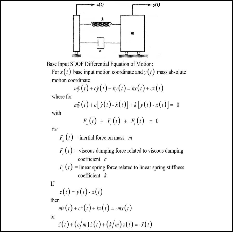
Figure description:
Key Information: Base Input SDOF System Model
- Model Components: Single Degree of Freedom (SDOF system featuring a mass (, a linear spring with stiffness (, and a viscous damper with coefficient (.
- Coordinates:
- : Base input motion coordinate.
- : Mass absolute motion coordinate.
- : Relative displacement between the mass and base.
- Forces:
- : Inertial force on mass .
- : Viscous damping force.
- : Linear spring force.
- Differential Equations of Motion:
- Absolute motion:
- Force equilibrium:
- Relative motion:
Figure 516.8-1. Base input SDOF system model for shock considerations.
MIL-STD-810H
METHOD 516.8
2.3.1.2 Laboratory Shock Test Options
The following paragraphs address the various options for conduct of laboratory shock tests. Consideration will be discussed regarding availability of field data.
2.3.1.2.1 Summary
For any configured materiel, ideally there exist “representative” field measurements of shock to which the materiel might be exposed during its life according to the LCEP. The eight procedures in this Method generally describe the scenarios in which field shock to materiel may occur. The procedures go beyond scenarios, and suggest default drop, default pulses, and/or default SRSs for applying laboratory shock. These “defaults” may have originated from field measurement data on some generic materiel in a particular configuration that were summarized and documented at one time, but this documentation no longer exists. Such lack of documentation leaves this Method with some procedures that are based upon the best laboratory test information currently available. The reality is that obtaining accurate item specific field measurements can be difficult, cost prohibitive, or not possible to acquire in a timely manner. However, to the maximum extent possible, tests based on measured data are the recommended option before use of the provided default test criteria.
NOTE: For materiel design and development, the option of tailoring of a laboratory shock test from field measurement information is superior to any of the test procedures within this Method, and should be the first laboratory test option. This assumes that the measurement data bandwidth and the laboratory test bandwidths are strictly compatible.
2.3.1.2.2 Test Implementation Options
Table 516.8-II summarizes the options for the eight laboratory test procedures. The options are defined as follows:
- a. “TWR” (Time Waveform Replication), means that the measurement time history will be reproduced on the laboratory exciter with “minimal amplitude time history error” according to Method 525.2 Typically implemented using special shock package software for replication.
- b. “Drop” is an explicit free fall drop event.
- c. “Classical Pulse” refers to classical pulses to be used in testing. Classical pulses defined within this method are the terminal peak sawtooth, trapezoidal and half-sine pulses. This category is generally employed when suitable field measurement information is unavailable, and traditional testing is relied upon.
- d. “SRS” refers to cases in which an SRS is used for the test specification, and exciter shock is synthesized based upon amplitude modulated sine waves or damped sinusoids. This category may be based on the SRS equivalent of a classical pulse to reduce adverse effects associated with conducting classical shock testing on a shaker, or may be defined based upon an ensemble of measured field data. The application notes in Annex A paragraph A.1.3 are important for defining the appropriate duration for the synthesized SRS pulse.
From Table 516.8-II, it is clear that the test procedures are divided according to use of TWR, drop test procedures, classical pulses, or synthesized waveforms from SRS. TWR is considered the most realistic as it is based upon direct replication of field measured data. Software vendors have generally incorporated an option for TWR within their “shock package,” so that it is unnecessary to plan testing under specialized TWR software as called out in Methods 525.2 and 527.2, however, both of these Methods provide insight into tolerance and scaling related to a more general TWR methodology.
| Procedure | Test Methodology | ||||||
|---|---|---|---|---|---|---|---|
| Drop1 | Classical Pulse | SRS | TWR | ||||
| Half- Sine2 | Trapezoidal | TP Sawtooth | |||||
| I | Functional Shock | X | X | X | X | ||
| II | Transportation Shock | X | X | X | |||
| III | Fragility | X | X | ||||
| IV | Transit Drop | X | |||||
| V | Crash Hazard Shock3 | X | X | X | |||
| VI | Bench Handling | X | |||||
| VII | Pendulum Impact4 | X | |||||
| VIII | Catapult Launch/ Arrested Landing5 | X | |||||
- Note 1. The Drop test includes vertical free fall towers, impact machines, and other test methods with similar equipment.
Note 2. High Speed Craft is a special case of Functional Shock that is specified in terms of classical half-sine.
Note 3. In some cases the Crash Hazard Shock may be evaluated by a constant acceleration, see paragraph 2.2.2e.
Note 4. Pendulum Impact is a test item with horizontal motion that impacts a stationary barrier.
Note 5. A Catapult Launch/Arrested Landing test can be based on a measured waveform or a two second damped (Q=20) sine burst of required amplitude and frequency, see the test procedure.
2.3.1.2.3 Tailoring When Measured Data Are Available - General Discussion
Since test tailoring to field measured data is considered a superior technique for shock testing, information and guidelines in this and subsequent paragraphs are very important. Beyond the classical pulse, two techniques of shock replication in the laboratory are possible.
- a. The first technique takes a measurement shock, and conditions it for direct waveform replication on the laboratory exciter. Conditioning may consist of bandwidth limiting via lowpass, highpass, or bandpass filtering, and re-sampling into an ASCII or other general file format. Vendor packages may have this capability within the “shock package” or in a special “Time Waveform Replication (TWR) package”.
- b. The second technique takes a measurement shock, computes an SRS estimate, and subsequently uses this SRS estimate to synthesize a representative time domain reference using a "wavelet" or a damped sine-based synthesis approach. In order to maintain a reasonable correlation between the effective pulse durations in the field measured and laboratory synthesized signals, in addition to the SRS reference to be synthesized, the test operator will require knowledge of the basic temporal characteristics of the time domain signal(s) from which the reference SRS is computed. More on this subject follows in Annex A Paragraph 1.3.
In summary, when test tailoring based upon available field measured data is employed, there are basically two laboratory test options available (assuming that repetition of the laboratory shock is under the guidance of the LCEP). Depending on the conditions of the test in which the data was acquired and the intended use for the data, the typical application of TWR or SRS test methods are described below.
- a. TWR.
- (1) Measured shock is a single shock field measurement or highly repeatable multiple shock field measurement.
- (2) Complex shocks.
- (3) Adequate measurement or ability to predict time histories at relevant locations in order to have adequate information at mounting locations of the test article.
- (4) Examples of such measurements are catapult launches, aircraft landing, and gunfire loads.
NOTE: The bandwidth of the measurement shock and the ability of the laboratory exciter system to “replicate the bandwidth” is an important consideration under TWR. TWR input time histories may be band-limited, and yet the materiel response may have broader bandwidth as a result of mounting. This area has not been studied to any extent, and can be a function of the materiel and its mounting. Time history bandwidths that exceed the laboratory exciter bandwidth place a rather severe limitation on use of TWR for laboratory testing.
b. SRS
- (1) Single or multiple shock measurements where SRS values fit to a statistical distribution. Confirmation of statistical trend must be made.
- (2) Sensor placement is sparse relative to the area in which it is to characterize.
- (3) The shock load is known to have a statistically high variance.
- (4) An example of SRS preference would be the shock assigned to a ground vehicle’s hull as a function of multiple terrains.
Scaling for conservatism is ill-defined, but may be applied at the discretion of the analyst.
NOTE: SRS synthesis requires not only the SRS estimate, but (1) a general amplitude correspondence with field measured or a predicted pulse, and (2) an estimate of the field measured or predicted pulse duration. In general, synthesis is applicable only for “simple shocks” (see Annex A paragraphs 1.2- 1.3) with high frequency information very near the peak amplitude, i.e., for shocks whose rms duration is short. By the nature of the composition of the synthesized shock (i.e., damped sinusoids or “wavelets”), it is possible to inappropriately extend the duration of a time history that matches a given SRS to an indefinitely long time. Note also that when measurement data are available, certain shocks, in particular “complex shocks” (see Annex B), may only be adequately applied under TWR.
2.3.2 Test Conditions
When defining shock test levels and conditions, every attempt needs to be made to obtain measured data under conditions similar to service environment conditions in the Life Cycle Environmental Profile. Consider the following test execution ranking from the most desirable to the least desirable as follows:
-
a. TWR: Measured time histories summarized, and laboratory exciter shock created by way of direct reproduction of one or more selected time histories under exciter waveform control (see Method 525).
-
b. SRS based on Measured Data: Measured time histories summarized in the form of an SRS and laboratory exciter shock synthesized by way of a complex transient making sure that effective shock durations ( and ) for the test pulse are consistent with the measured data and the character of the synthesized waveform is “similar” to the measured time histories with respect to amplitude and zero crossings (see Annex A Paragraph 1.3 for a discussion and example of effective shock durations).
-
c. SRS in the absence of Measured Data: No measured time histories but previous SRS estimates available, and laboratory exciter shock synthesized by way of a complex transient such that effective shock durations ( and ) are specified taking into consideration the nature of the environment and the natural frequency response characteristics of the materiel (see Annex A Paragraphs 1.3 and 1.4).
-
d. Classical Shock Pulse: No measured time histories, but classical pulse shock descriptions available for use in reproducing the laboratory exciter shock (see Paragraph 2.3.2.3).
2.3.2.1 SRS Based on Measured Data
When measured data is available, the SRS required for the test will be determined from analytical computations. and required for the test will be determined from statistical processing of time history measurements of the materiel’s environment (see Annex A, Paragraph 1.3). Unless otherwise specified, the SRS analysis will be performed on the AC coupled time history for at a sequence of natural frequencies spaced at 1/12 octave or less to span a minimum bandwidth of 5 Hz to 2,000 Hz.
- a. When a sufficient number of representative shock spectra are available, employ an appropriate statistical enveloping technique to determine the required test spectrum with a statistical basis (see Annex C of this Method).
- b. When insufficient measured time histories are available for statistical analysis (only one or two time histories of like character), use an increase over the maximum of the available SRS spectra to establish the required test spectrum (if two spectra are available, determine a maximum envelope according to the ENV procedure of Annex C). The resulting spectra should account for stochastic variability in the environment, and uncertainty in any predictive methods employed. The degree of increase over measured time history spectra is based on engineering judgment, and should be supported by rationale. In these cases, it is often convenient to add either a 3 dB or 6 dB margin to the enveloped SRS, depending on the degree of test level conservatism desired (see Annex C, paragraph 4.2). Effective durations and for test should be taken as the respective maximums as computed from each of the measured time histories.
2.3.2.2 SRS in the Absence of Measured Data
If measured data is not available, the SRS and the corresponding values of and may be derived from (1) a carefully scaled measurement of a dynamically similar environment, (2) structural analysis or other prediction methods, or (3) from a combination of sources. For Procedure I (Functional Shock with Terminal Peak Sawtooth Reference Criteria), and Procedure V (Crash Hazard Shock), employ the applicable SRS spectrum from Figure 516.82 as the test spectrum for each axis, provided and of the test shock time history is in compliance with the accompanying Table 516.8-III. This spectrum approximates that of the perfect terminal-peak sawtooth pulse. General guidance for selecting the crossover frequency, , for any classical pulse is to define it as the lowest frequency at which the corresponding SRS magnitude reaches the convergence magnitude (the constant magnitude reached in the high frequency portion of the SRS) for the damping ratio of interest. Once is defined, the effective duration considered in the complex pulse synthesis is then defined as . This guidance allows for a longer effective duration than previous versions of this standard that were found to be too restrictive. Refer to Annex A paragraph 1.3 for additional guidance on customizing the bandwidth of the SRS and corresponding values of and as required.
It is recommend that the test be performed with a waveform that is synthesized from either (1) a superposition of damped sinusoids with selected properties at designated frequencies, or (2) a superposition of various amplitude modulated sine waves with selected properties at designated frequencies, such that this waveform has an SRS that
approximates the SRS on Figure 2. In reality, any complex test transient with major energy in the initial portion of the time trace is suitable if it is within tolerance of this spectrum requirement over the minimum frequency range of 10 to 2000 Hz, and meets the duration requirements. Implementing a classical terminal-peak sawtooth pulse or trapezoidal pulse on a vibration exciter are the least permissible test alternatives. In the case in which a classical pulse is given as the reference criteria, it is permissible to synthesize a complex pulse based on the SRS characteristics of the referenced classical pulse. In such cases, and should be defined as in Table 516.8-III.
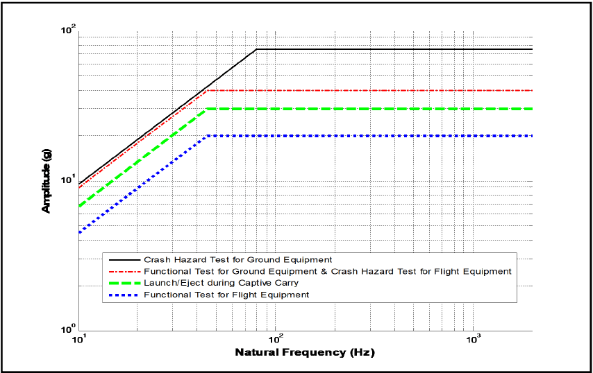
Figure description:
Amplitude (g vs Natural Frequency (Hz
Legend
- Crash Hazard Test for Ground Equipment — color: black; symbol: Solid line
- Functional Test for Ground Equipment & Crash Hazard Test for Flight Equipment — color: red; symbol: Dash-dotted line
- Launch/Eject during Captive Carry — color: green; symbol: Dashed line
- Functional Test for Flight Equipment — color: blue; symbol: Dotted line
| Natural Frequency (Hz) | Crash Hazard Test for Ground Equipment (g) | Functional Test for Ground Equipment & Crash Hazard Test for Flight Equipment (g) | Launch/Eject during Captive Carry (g) | Functional Test for Flight Equipment (g) |
|---|---|---|---|---|
| 10 | 10.0 | 8.9 | 6.7 | 4.4 |
| 45 | 45.0 | 40.0 | 30.0 | 20.0 |
| 75 | 75.0 | 40.0 | 30.0 | 20.0 |
| 100 | 75.0 | 40.0 | 30.0 | 20.0 |
| 1000 | 75.0 | 40.0 | 30.0 | 20.0 |
| 2000 | 75.0 | 40.0 | 30.0 | 20.0 |
Notes: The data is plotted on a log-log scale. All four series follow a +1 slope (in log-log coordinates from the starting frequency of 10 Hz until reaching their respective plateau levels. The series for 'Crash Hazard Test for Ground Equipment' reaches its plateau of 75g at approximately 75 Hz. The other three series ('Functional Test for Ground Equipment & Crash Hazard Test for Flight Equipment', 'Launch/Eject during Captive Carry', and 'Functional Test for Flight Equipment' all reach their respective plateaus of 40g, 30g, and 20g at a common frequency of approximately 45 Hz.))
Figure 516.8-2. Test SRS for use if measured data are not available (for Procedure I - Functional Shock, and Procedure V - Crash Hazard Shock).
| Test Category | Peak Acceleration (G-Pk) | Te (ms)1 | TE (ms)1 | Cross-over Frequency Fco (Hz) |
|---|---|---|---|---|
| Functional Test for Flight Equipment | 20 | 2.5/ fmin | 2/Fco | 45 |
| Functional Test for Ground Equipment2 | 40 | 2.5/ fmin | 2/Fco | 45 |
| Launch/Eject During Captive Carry | 30 | 2.5/ fmin | 2/Fco | 45 |
| Crash Hazard Shock Test for Flight Equipment | 40 | 2.5/ fmin | 2/Fco | 45 |
| Crash Hazard Shock Test for Ground Equipment | 75 | 2.5/ fmin | 2/Fco | 80 |
Note 1: The default value for is 10 Hz as shown in Figure 516.8-2. Refer to guidance in paragraphs 4.2.2.2.c and 4.2.2.2.d to customize the bandwidth of the SRS and corresponding values of and .
Note 2. For materiel mounted only in trucks and semi-trailers, use a 20G peak value.
MIL-STD-810H METHOD 516.8
516.8-2.3.2 NPL - Upper Normal Prediction limit
The upper normal prediction limit (NPL) is the value of x (for the original data set) that will exceed the next predicted or measured value with confidence coefficient, Y, and is given by
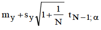
Figure description:
1 my+Sy₁ 1+ tN-la N
where . is the student distribution variable with N-1 degrees of freedom at the percentage point of the distribution. This estimate, because of the assumptions behind its derivation, requires careful interpretation relative to measurements made in a given location or over a given estimate zone (paragraph 6.1 , reference b).
2.3.2.3 Classical Shock Pulse
Classical shock pulses (e.g., half-sine, terminal peak sawtooth, or trapezoidal) may be defined by (1) time history measurements of the materiel's environment, (2) from a carefully scaled measurement of a dynamically similar environment, (3) from structural analysis or other prediction methods, or (4) from a combination of sources. The terminal peak sawtooth is often referenced due to its relatively flat spectral characteristics in the SRS domain as approximated in Figure 516.8-2. In the event that a-priori information regarding rise time of the transient event being considered is determined to be a critical parameter, consider a half-sine pulse or a trapezoidal pulse with a tailored rising edge in lieu of the terminal peak sawtooth. Shock pulse substitution (e.g., half-sine in lieu of terminal peak sawtooth) requires adjustment in the amplitude such that the velocity of the substituted shock pulse is equivalent to the original specification. The resulting over-test or under-test with respect to the difference in the SRS must be considered, documented, and approved by the appropriate testing authority. If a classical shock pulse is defined in lieu of more complex measured time history data it must be demonstrated that SRS estimates of the classical shock pulse are within the tolerances established for the SRS estimates of the measured time history data. In most cases, classical shock pulses will be defined as one of the following:
- a. Terminal Peak Sawtooth Pulse: The terminal peak sawtooth pulse along with its parameters and tolerances are provided in Figure 516.8-3, and is an alternative for testing in Procedure I - Functional Shock, Procedure II - Transportation Shock and Procedure V - Crash Hazard Shock Test.
- b. Trapezoidal Shock Pulse: The trapezoidal pulse along with its parameters and tolerances is provided in Figure 516.8-4. The trapezoidal pulse is specified for Procedure III - Fragility.
- c. Half-Sine Shock Pulse: The half-sine pulse along with its parameters and tolerances is provided in Figure 516.8-5. The Half-Sine Pulse is specified for Procedure I – High Speed Craft Functional Shock. As discussed in paragraph 2.3.2.3.1, the half-sine pulse is often used in lieu of other classical pulses based upon equipment availability and or limitations.
MIL-STD-810H METHOD 516.8
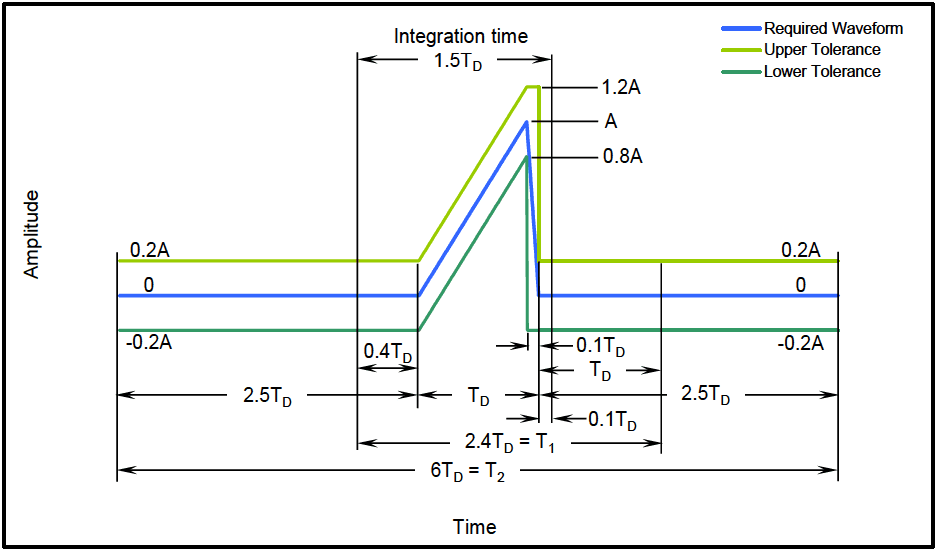
Figure description:
Waveform Amplitude vs Time
Legend
- Required Waveform — color: blue; symbol: Solid line
- Upper Tolerance — color: light green; symbol: Solid line
- Lower Tolerance — color: dark green; symbol: Solid line
Annotations
- Integration time 1.5T_D (text_label - position: x = 2.5T_D to 4.0T_D)
- 2.4T_D = T_1 (text_label - position: x = 2.5T_D to 4.9T_D)
- 6T_D = T_2 (text_label - position: x = 0 to 6.0T_D)
- 0.4T_D (text_label - position: x = 2.5T_D to 2.9T_D)
- T_D (text_label - position: x = 2.9T_D to 3.9T_D)
- 0.1T_D (text_label - position: x = 3.9T_D to 4.0T_D)
- T_D (text_label - position: x = 4.0T_D to ~5.0T_D)
| Time | Required Waveform (Amplitude) | Upper Tolerance (Amplitude) | Lower Tolerance (Amplitude) |
|---|---|---|---|
| 0 | 0 | 0.2A | -0.2A |
| 2.5T_D | 0 | 0.2A | -0.2A |
| 2.5T_D + 0.4T_D | 0 | 0.2A | -0.2A |
| 2.5T_D + 0.4T_D + T_D | A | 1.2A | 0.8A |
| 2.5T_D + 0.4T_D + T_D (immediately after) | 0 | 1.2A | -0.2A |
| 2.5T_D + 0.4T_D + T_D + 0.1T_D | 0 | 1.2A | -0.2A |
| 2.5T_D + 0.4T_D + T_D + 0.1T_D (immediately after) | 0 | 0.2A | -0.2A |
| 2.5T_D + T_1 | 0 | 0.2A | -0.2A |
| T_2 | 0 | 0.2A | -0.2A |
Notes: The chart illustrates a pulse waveform with its upper and lower tolerance limits. The timing is parameterized by T_D and the amplitude by A. There are some slight inconsistencies in the visual scale labels (e.g., 2.5T_D + 2.4T_D + 2.5T_D = 7.4T_D, yet the total T_2 is labeled as 6T_D. The data table follows the explicit segment labels.)
Figure 516.8-3. Terminal peak sawtooth shock pulse configuration and its tolerance limits.
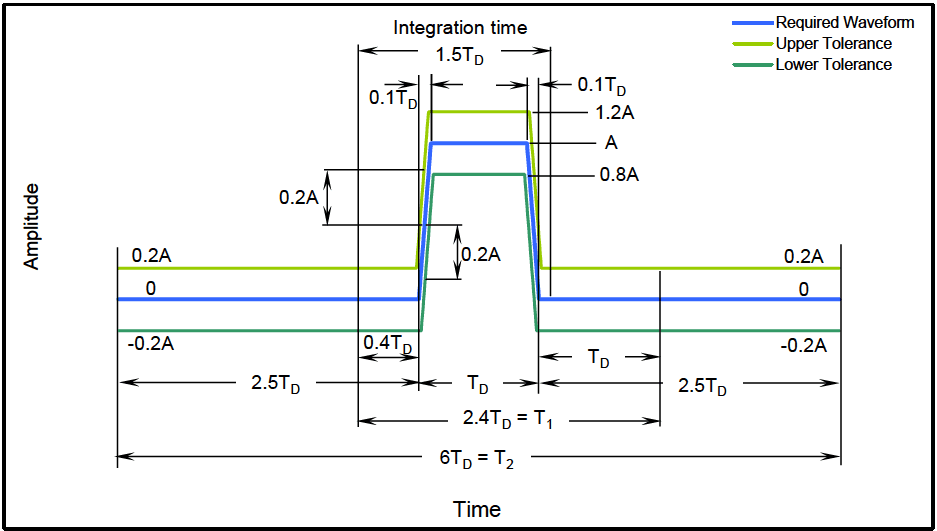
Figure description:
Signal Tolerance Definitions
Waveform and Tolerance Mask
Legend
- Required Waveform — color: blue; symbol: solid line
- Upper Tolerance — color: light green; symbol: solid line
- Lower Tolerance — color: dark green; symbol: solid line
Annotations
- Integration time = 1.5TD (horizontal_interval - position: t = 2.2TD to 3.7TD)
- T1 = 2.4TD (horizontal_interval - position: t = 2.1TD to 4.5TD)
- T2 = 6TD (horizontal_interval - position: t = 0 to 6.0TD)
- Required pulse width = TD (horizontal_interval - position: t = 2.5TD to 3.5TD)
- Upper Tolerance Peak = 1.2A (text_label - position: y = 1.2A)
- Required Peak = A (text_label - position: y = A)
- Lower Tolerance Peak = 0.8A (text_label - position: y = 0.8A)
- Vertical Tolerance = 0.2A (text_label - position: gap between waveforms)
- Horizontal Tolerance = 0.1TD (text_label - position: offset between blue and upper tolerance corners)
| Time () | Required Waveform () | Upper Tolerance () | Lower Tolerance () |
|---|---|---|---|
| 0.0 | 0.0 | 0.2 | -0.2 |
| 2.1 | 0.0 | 0.2 | -0.2 |
| 2.4 | 0.0 | 1.2 | -0.2 |
| 2.5 | 1.0 | 1.2 | 0.8 |
| 3.5 | 1.0 | 1.2 | 0.8 |
| 3.6 | 0.0 | 0.2 | -0.2 |
| 4.5 | 0.0 | 0.2 | -0.2 |
| 6.0 | 0.0 | 0.2 | -0.2 |
Notes: The chart shows a pulsed waveform with its upper and lower tolerance limits. The horizontal axis is normalized to the pulse duration TD, and the vertical axis is normalized to the required peak amplitude A. The total window shown is 6TD. A specific integration time of 1.5TD is also indicated.
Figure 516.8-4. Trapezoidal shock pulse configuration and tolerance limits.
MIL-STD-810H METHOD 516.8
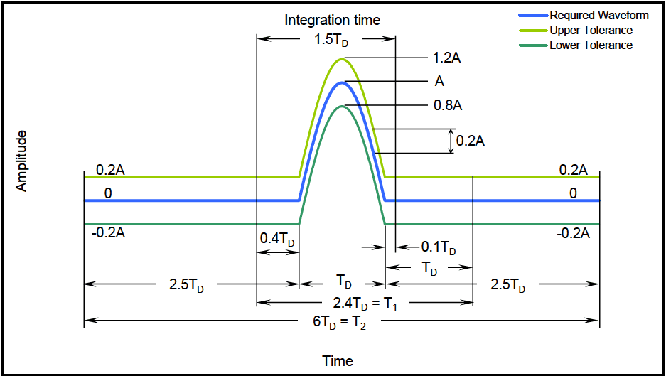
Figure description:
Waveform and Tolerance Limits
Amplitude vs Time Waveform Specification
Legend
- Required Waveform — color: blue; symbol: Solid line
- Upper Tolerance — color: light green; symbol: Solid line
- Lower Tolerance — color: dark green; symbol: Solid line
Annotations
- Integration time (text_label - position: Centered above the pulse)
- 1.5 (horizontal_span - position: From t = 2.1 to t = 3.6 )
- 2.4 (horizontal_span - position: From t = 2.1 to t = 4.5 )
- 6 (horizontal_span - position: From t = 0 to t = 6.0 )
- (horizontal_span - position: Pulse width at base from t = 2.5 to t = 3.5 )
- (right (horizontal_span - position: From t = 3.5 to t = 4.5 ))
- 0.4 (horizontal_span - position: From t = 2.1 to t = 2.5 )
- 0.1 (horizontal_span - position: From t = 3.5 to t = 3.6 )
- 2.5 (left (horizontal_span - position: Baseline duration from t = 0 to t = 2.5 ))
- 2.5 (right (horizontal_span - position: Baseline duration from t = 3.5 to t = 6.0 ))
- 1.2A (text_label - position: Peak of Upper Tolerance at t = 3.0 )
- A (text_label - position: Peak of Required Waveform at t = 3.0 )
- 0.8A (text_label - position: Peak of Lower Tolerance at t = 3.0 )
- 0.2A (vertical_span - position: Tolerance band amplitude offset)
| Time | Required Waveform | Upper Tolerance | Lower Tolerance |
|---|---|---|---|
| 0 | 0 | 0.2A | -0.2A |
| 2.1 | 0 | 0.2A | -0.2A |
| 2.5 | 0 | 0.2A | -0.2A |
| 3.0 | A | 1.2A | 0.8A |
| 3.5 | 0 | 0.2A | -0.2A |
| 3.6 | 0 | 0.2A | -0.2A |
| 4.5 | 0 | 0.2A | -0.2A |
| 6.0 | 0 | 0.2A | -0.2A |
Notes: The chart defines a pulsed waveform with specific timing () and amplitude () parameters, including tolerance bounds of +/- 0.2A.
Figure 516.8-5. Half-Sine shock pulse configuration and tolerance limits.
Key to Figures 516.8-3 through 516.8-5:
- TD: duration of nominal pulse (tolerance on TD is ±10%).
- A: peak acceleration of nominal pulse
- T₁: minimum time duration which the pulse shall be monitored for shocks produced using a conventional mechanical shock machine.
- T2: minimum time during which the pulse shall be monitored for shocks produced using a vibration exciter.
The duration associated with the post-pulse slope of a terminal peak sawtooth and durations associated with the pre and post slopes of a trapezoidal pulse should be less than 10% TD.
The tolerance on velocity, due to combined effects of any amplitude and/or duration deviations from the nominal pulse, is limited to +/- 20% of the pulse's nominal velocity.
2.3.2.3.1 Classical Shock Pulses (Mechanical Shock Machine)
It is recognized that conducting a terminal peak sawtooth or trapezoidal pulse on a mechanical shock machine requires the use of special programmers (e.g., lead or gas programmers) and requires higher impact velocity than equivalent half-sine shocks since the half-sine pulse contains significant rebound velocity that is not characteristic of the terminal peak sawtooth pulse. Such programmers or high velocity shock machines are not available in all laboratories. In such cases, it may be necessary to resort to the use of more readily available programmers used in the conduct of half-sine shock pulses. When substitution of shock pulses is necessary, follow the general guidance of maintaining equivalent velocity to that of the original reference pulse.
2.3.2.3.2 Classical Shock Pulses (Vibration Exciter)
If a vibration exciter is to be employed to conduct a test with a classical shock pulse, it will be necessary to optimize the reference pulse such that the net velocity and displacements are zero. Unfortunately, the need to compensate the reference pulse distorts the temporal and spectral characteristics, resulting in two specific problems that will be illustrated through example using a terminal peak sawtooth (the same argument is relevant for any classical pulse test to be conducted on a vibration exciter). First, any pre and/or post-pulse compensation will be limited by the +20
percent tolerances given in Figures 516.8-3 to 516.8-5. Second, as illustrated by the pseudo-velocity SRS in Figure 516.8-6, the velocities in the low frequency portion of the SRS will be significantly reduced in amplitude. Also, there is generally an area of increased amplitude associated with the duration of the pre- and post-test compensation. Observe that the low frequency drop-off in SRS levels between the compensated and uncompensated pulse is readily identifiable and labeled . Likewise, the frequency at which the compensated and uncompensated pulses converge is readily identifiable and labeled . The drop-off at is considered to be acceptable if and only if the lowest resonant frequency of the item being tested, , is at least one octave greater than . The amount of gain in the region is directly related to the duration and magnitude of the compensation pulse and the percent of critical damping employed in the SRS computation (Q=10 in Figure 516.8-6). The potential for over-test in this spectral band must also be carefully considered prior to proceeding.
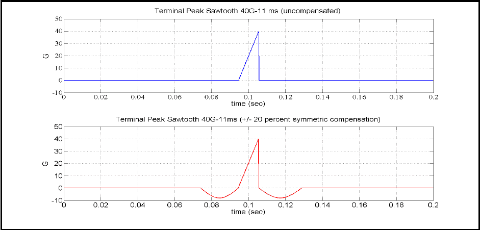
Figure description:
Shock Pulse Profiles: Uncompensated vs. Compensated
Terminal Peak Sawtooth 40G-11 ms (uncompensated
| time (sec) | G |
|---|---|
| 0.000 | 0.0 |
| 0.094 | 0.0 |
| 0.105 | 40.0 |
| 0.105 | 0.0 |
| 0.200 | 0.0 |
Terminal Peak Sawtooth 40G-11ms (+/- 20 percent symmetric compensation
| time (sec) | G |
|---|---|
| 0.000 | 0.0 |
| 0.073 | 0.0 |
| 0.078 | -5.7 |
| 0.083 | -8.0 |
| 0.089 | -5.7 |
| 0.094 | 0.0 |
| 0.105 | 40.0 |
| 0.105 | 0.0 |
| 0.110 | -5.7 |
| 0.116 | -8.0 |
| 0.121 | -5.7 |
| 0.127 | 0.0 |
| 0.200 | 0.0 |
Notes: The figure illustrates shock pulse profiles used in mechanical testing. The top chart shows a standard uncompensated terminal peak sawtooth pulse with a peak acceleration of 40G and a duration of 11ms. The bottom chart displays the same pulse with symmetric compensation to achieve zero net velocity change; the compensation pulses have a peak magnitude of -8G (20% of the main pulse and are positioned immediately before and after the main shock pulse.)
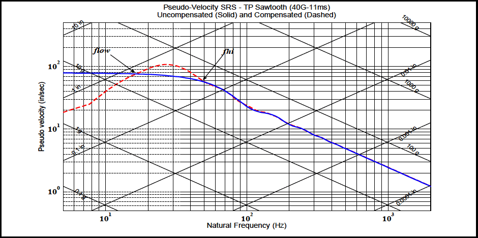
Figure description:
Pseudo-Velocity SRS - TP Sawtooth (40G-11ms Uncompensated (Solid and Compensated (Dashed
Pseudo-Velocity SRS - TP Sawtooth (40G-11ms
Legend
- Uncompensated — color: blue; symbol: Solid line
- Compensated — color: red; symbol: Dashed line
Annotations
- flow (text_label - position: x ≈ 18 Hz, y ≈ 78 in/sec)
- fhi (text_label - position: x ≈ 55 Hz, y ≈ 55 in/sec)
| Natural Frequency (Hz) | Uncompensated (Solid Blue (in/sec)) | Compensated (Dashed Red (in/sec)) |
|---|---|---|
| 5 | 80.0 | 18.0 |
| 6 | 80.0 | 20.0 |
| 8 | 80.0 | 25.0 |
| 10 | 80.0 | 35.0 |
| 15 | 78.0 | 65.0 |
| 18 | 76.0 | 80.0 |
| 20 | 75.0 | 90.0 |
| 25 | 72.0 | 105.0 |
| 30 | 70.0 | 102.0 |
| 40 | 65.0 | 82.0 |
| 50 | 58.0 | 62.0 |
| 60 | 50.0 | 50.0 |
| 80 | 35.0 | 35.0 |
| 100 | 25.0 | 25.0 |
| 150 | 18.0 | 18.0 |
| 200 | 12.0 | 12.0 |
| 300 | 8.5 | 8.5 |
| 500 | 4.8 | 4.8 |
| 1000 | 2.5 | 2.5 |
| 1500 | 1.8 | 1.8 |
| 2500 | 1.1 | 1.1 |
Notes: The chart is a four-coordinate plot with primary axes for Natural Frequency (Hz and Pseudo Velocity (in/sec and auxiliary diagonal grid lines for Acceleration (g and Displacement (in. All axes are logarithmic.))))
Figure 516.8-6. Illustration of temporal and spectral distortion associated with a compensated classical terminal peak sawtooth.
MIL-STD-810H
METHOD 516.8
2.3.3 Test Axes and Number of Shock Events - General Considerations
Generally, the laboratory test axes and the number of exposures to the shock events should be determined based upon the LCEP. However as a minimum requirement, subject the test item to a sufficient number of suitable shocks to meet the specified test conditions in both directions along each of three orthogonal axes. A suitable test shock for each direction of each axis is defined to be one classical shock pulse or complex transient pulse that yields a response spectrum that is within the tolerances of the required test spectrum over the specified frequency range, and has an effective duration within the tolerance of as defined in paragraph 4.2.2.2. In general, complex transient pulses generated by modern control systems will be symmetric and the maximax positive and negative SRS levels will be the same. However, this must be verified for each shock event by computing the spectra for positive and negative maximum (i.e., maximum and minimum) accelerations, generally at , and at least 1/12-octave frequency intervals. If the required test spectrum can be satisfied simultaneously in both directions along an axis (i.e., symmetric pulse), one shock event will satisfy a single shock requirement for that axis in both directions. If the requirement can only be satisfied in one direction (e.g., polarity consideration for classical shock inputs, non-symmetric complex transient pulses), it is permissible to change the test setup and impose an additional shock to satisfy the spectrum requirement in the other direction. This may be accomplished by either reversing the polarity of the test shock time history or reversing the test item orientation. The following guidelines may also be applied for either classical shock pulses or complex transient pulses.
a. For materiel that is likely to be exposed only rarely to a given shock event, perform a minimum of one shock in each direction of each axis. For shock conditions with a high potential of damage (e.g., large velocity change associated with the shock event, fragile test article), perform no more than one shock in each direction of each axis. Note that some high velocity shock tests with safety implications (i.e., crash hazard) may require two shocks in each direction of each axis.
b. For materiel likely to be exposed more frequently to a given shock event, and there are little available data to substantiate the number of shocks, apply a minimum of three shocks in each direction of each axis.
2.3.3.1 Special Considerations for Complex Transients
There is no unique synthesized complex transient pulse satisfying a given SRS. In synthesizing a complex transient pulse from a given SRS, and this complex transient pulse either (1) exceeds the capability of the shock application system (usually in displacement or velocity), or (2) the duration of the complex transient pulse is more than 20 percent longer than T , some compromise in spectrum or duration tolerance may be necessary. It is unacceptable to E decompose an SRS into a low frequency component (high velocity and displacement), and a high frequency component (low velocity and displacement) to meet a shock requirement. Often an experienced analyst may be able to specify the input parameters to the complex transient pulse synthesis algorithm in order to satisfy the requirement for which the shock application system manufacturer “optimum” solution will not. Refer to paragraphs 4.2.2.2.c and 4.2.2.2.d.
2.4 Test Item Configuration
(See Part One, paragraph 5.8.) The configuration of the test item strongly affects test results. Use the anticipated configuration of the materiel in the life cycle environmental profile. As a minimum, consider the following configurations:
- a. In a shipping/storage container or transit case.
- b. Deployed in the service environment.
516.8-2.4 Non-parametric Upper Limit Statistical Estimate Procedures
If there is some reason to believe that the estimate at a given frequency, after they have been logarithm-transformed, will not be sufficiently normally distributed to apply the parametric limits defined above, consideration must be given to nonparametric limits, i.e., limits that are not dependent upon assumptions concerning the distribution of estimate values. In this case there is no need to transform the data estimates. All of the assumptions concerning the selection of estimates are applicable for nonparametric estimates. With additional manipulation, lower bound limits may be computed.
2.4.1 Envelope (ENV) - Upper Limit
The maximum upper limit is determined by selecting the maximum estimate value in the data set.
ENV(N) = max{X1, X2, XN }
The main disadvantage of this estimate is that the distributional properties of the estimate set are neglected, so that no probability of exceedance of this value is specified. In the case of outliers in the estimate set, ENV(N) may be far too conservative. ENV(N) is also sensitive to the bandwidth of the estimates.
2.4.2 Distribution Free Limit (DFL) - Upper Distribution-Free Tolerance Limit
The distribution-free tolerance limit that uses the original untransformed sample values is defined to be the upper limit for which at least the fraction of all sample values will be less than the maximum predicted or measured value with a confidence coefficient of " ". This limit is based on order statistic considerations.
DEL(N,B,y)=Xmax;}=1-BN
where Xmax is the maximum value of the set of estimates, ẞ, is the fractional proportion below Xmax, and y is the confidence coefficient. N, ẞ and y are not independently selectable. That is
- a. Given N and assuming a value of ẞ, 0 ≤ẞ≤ 1, the confidence coefficient can be determined.
- b. Given N and y, the proportion ẞ can be determined.
- c. Given and , the number of samples can be determined such that the proportion and confidence can be satisfied (for statistical experiment design).
DFL(N,ẞ,y) may not be meaningful for small samples of data, N≤13, and comparatively large ẞ, ẞ>0.95. DFL (N,ẞ,y) is sensitive to the estimate bandwidth.
MIL-STD-810H
METHOD 516.8 ANNEX C
2.4.3 Empirical Tolerance Limit (ETL) - Upper Empirical Tolerance Limit
The empirical tolerance limit uses the original sample values and assumes the predicted or measured estimate set is composed of N measurement points over M frequency analysis bandwidths, for a total of NM estimate values. That is
{x11, X12, ..., X1M; X21, X22, ..., X2M; XN1, XN2, XNM}
where mj ¡ is the average estimate at the jth frequency bandwidth over all N measurement points
1 N mj = ΣΧ j = 1, 2, , M Ni=1
m; is used to construct an estimate set normalized over individual frequency resolution bandwidths. That is {u} = {u11, 12, , U1M, U21, U22, ..., U2M, UN1, UN2, , UNM}
where: Uhij = Xij i=1, 2, ..., N; j = 1, 2, ..., M mj
The normalized estimate set, {u}, is ordered from smallest to largest and uẞ = u() where uα) is the kth ordered element k of set {u} for 0 <ẞ= <1 is defined. For each resolution frequency bandwidth, then MN
ETL(B)=uẞm; = xẞj j = 1, 2, , M
Using my implies that the value of ETL(ẞ) at j exceeds ẞ percent of the values with 50 percent confidence. If a value other than m, is selected, the confidence level may increase. It is important that the set of estimates is homogeneous to use this limit, i.e., they have about the same spread in all frequency bands. In general, apply this limit only if the number of measurement points, N, is greater than 10.