3definitions

MIL-STD-810H

PART ONE ANNEX C

Figure description:

Map Subject: Global distribution of climatic categories based on MIL-STD-810H standards.

Climatic Categories (Legend:

• A1 EXTREME HOT DRY: Darkest orange/brown (primarily Sahara, Arabian Peninsula, parts of Central Asia/India, and Australian Outback.
• A2 HOT DRY: Medium orange (fringes of A1 zones, parts of Mexico/Southwest USA, and Southern Africa.
• A1 Hot Dry: Reddish-orange (smaller pockets within hot regions.
• A2 Basic Hot: Light orange/tan (widely distributed across equatorial and subtropical regions.
• A3 Intermediate: Yellow (temperate and northern/southern latitudes.

Key Regional Highlights:

• North America: Hot zones concentrated in the Southwest USA and Mexico.
• South America: Small hot pockets in northern Argentina and parts of Brazil.
• Africa/Middle East: Contains the largest contiguous area of "Extreme Hot Dry" (A1 and "Hot Dry" (A2 climates, spanning the Sahara to the Persian Gulf.
• Asia: Significant hot zones in India, Pakistan, and Western China/Central Asia.
• Australia: Central and western regions are predominantly "Extreme Hot Dry" and "Hot Dry."
• Unshaded Areas: Polar regions (Arctic/Antarctica and high northern latitudes are not categorized under these specific hot/dry labels.

MIL-STD-810H

PART ONE ANNEX

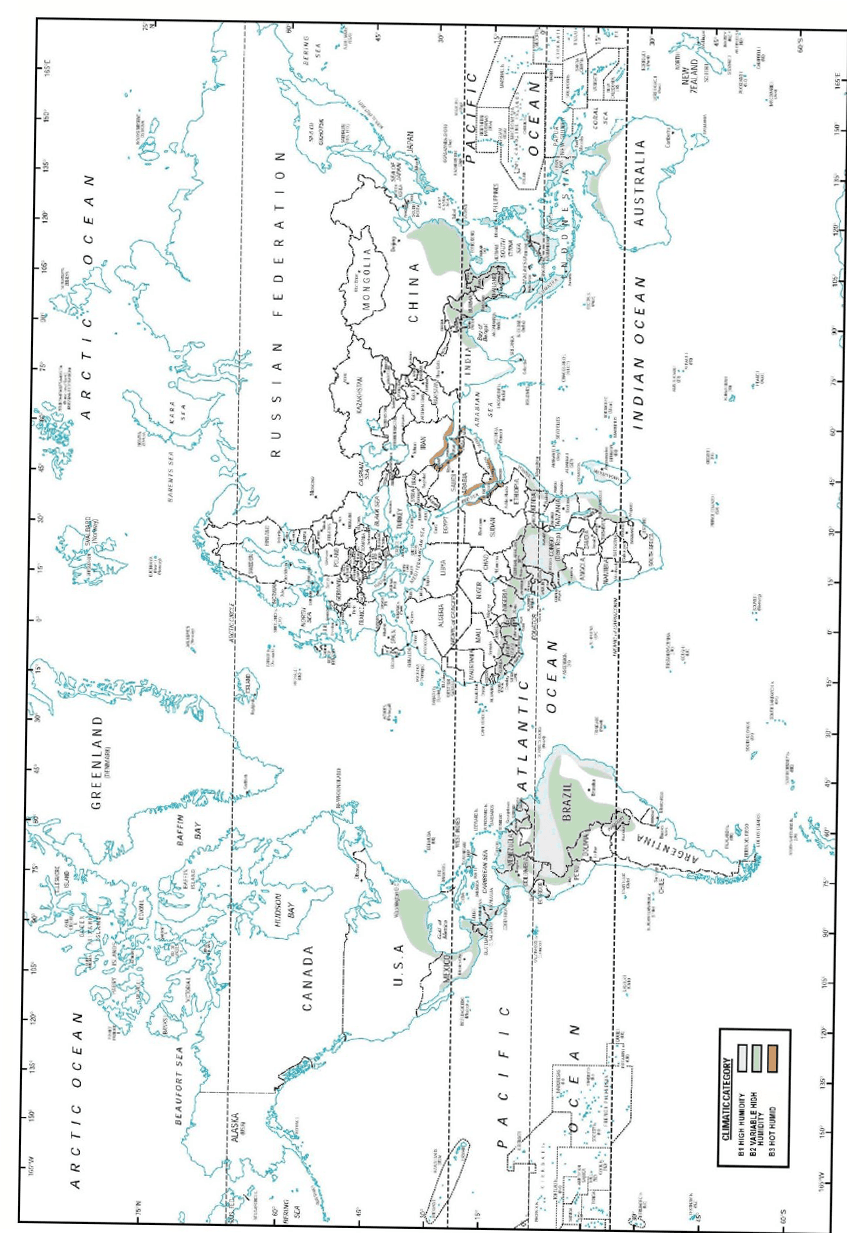
Figure description:

• Document Source: MIL-STD-810H, Part One, Annex C.
• Subject: World map illustrating the global distribution of specific climatic categories.
• Climatic Categories (Legend:
  • B1 High Humidity (Green: Concentrated in equatorial regions including the Amazon Basin, Congo Basin, Southeast Asia, and northern Australia.
  • B2 Variable High Humidity (Blue-green: Surrounds B1 zones, extending further into South America, Africa, and East Asia.
  • B3 Hot Humid (Orange: Predominantly follows tropical and subtropical coastlines and includes various island chains in the Pacific and Indian Oceans.
• Key Entities: North and South America, Africa, Eurasia, Australia, and major oceans (Pacific, Atlantic, Indian, Arctic.

PART ONE-C-6

MIL-STD-810H PART ONE ANNE

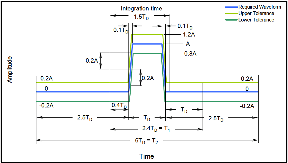
Figure description:

Global Distribution of Climatic Categories

CLIMATIC CATEGORY

Legend

• C0 Mild Cold — color: white; symbol: solid rectangle
• C1 Basic Cold — color: lightest blue; symbol: solid rectangle
• C2 Cold — color: light blue; symbol: solid rectangle
• C3 Severe Cold — color: medium blue/purple; symbol: solid rectangle
• C4 Extreme Cold — color: dark purple; symbol: solid rectangle

PART ONE C 7

Table C-I. Summary of climatic conditions and daily cycles of temperature, solar radiation, and relative humidity

• ¹ Designations in parentheses refer to corresponding climatic categories in MIL-HDBK-310 and AR-70-38 (except the A-3 category) and NATO STANAG 4370, AECTP 230; (see Part One, 2.2.1, 2.2.2, and 2.3).
• ² °C values (rounded to the nearest whole degree) derived from data obtained/established on °F scale.
• ³ Bph represents British Thermal Units per square foot per hour.
• 4 Sequence of RH presentation corresponds to sequence of air temperatures shown (e.g., for HOT-DRY daily cycle, 8 percent RH occurs at 32°C (90°F); 3 percent RH occurs at 49°C (120°F).
• ^5 Relative humidity for the A3 storage condition vary to widely between different situations to be represented by a single set of conditions.
• 6 Values are only found in NATO STANAG 4370, AECTP 230.
• 7 Delineation to be used for natural environment exposure testing, not applicable to laboratory testing.

NOTE: The numbers shown for the values of the climatic elements represent only the upper and lower limits of the cycles that typify days during which the extremes occur; e.g., for the Hot-Dry cycle, 49°C (120°F) is the maximum daytime temperature, and 32°C (90°F) is the minimum nighttime (or early morning) temperature.

MIL-STD-810H

PART ONE ANNEX C

Table C-II. Summary of potential environments for the STORAGE PHASE

Table C-III. Summary of potential environments for the TRANSPORTATION PHASE

MIL-STD-810H

PART ONE ANNEX C

Table C-III (Con't). Summary of potential environments for the TRANSPORTATION PHASE

Table C-IV. Summary of potential environments for the DEPLOYMENT PHASE

MIL-STD-810H

PART ONE ANNEX C

Table C-IV (Con’t). Summary of potential environments for the DEPLOYMENT PHASE

MIL-STD-810H

PART ONE ANNEX C

Table C-IV (Con't). Summary of potential environments for the DEPLOYMENT PHASE

MIL-STD-810H

PART ONE ANNEX D

PART ONE ANNEX D¹ TERMINOLOGY FOR DYNAMIC (MECHANICAL) TEST METHODS

• a. AC-coupling. In signal processing, this term implies the removal of any zero frequency information from the time history trace. In digitizing a signal, the analog-to-digital converter is said to be AC-coupled, if there exists a high pass filter in the digitizing process. Typically, piezoelectric devices are AC-coupled because of their inability to respond to static voltages.
• b. Autocorrelation function. For x(t), a function of time, the autocorrelation function, $R_{x x}(\tau)$, is defined to be the following average over an averaging time, T,

$\mathrm{R}_{\mathrm{xx}}(\tau)=\frac{1}{\mathrm{~T}} \int_{0}^{\mathrm{~T}} \mathrm{x}(\mathrm{t}) \mathrm{x}(\mathrm{t}+\tau) \mathrm{dt}$

If the average $\mathrm{R}_{\mathrm{xx}}(\tau)$ is also a function of time, t, $\left(\mathrm{R}_{\mathrm{xx}}(\tau, \mathrm{t})\right)$ such that

$\mathrm{R}_{\mathrm{xx}}(\tau, \mathrm{t})=\frac{1}{\mathrm{~T}} \int_{\mathrm{T}} \mathrm{x}(\mathrm{t}+\mathrm{u}) \mathrm{x}(\mathrm{t}+\mathrm{u}+\tau) \mathrm{du}$

then, this is a form of nonstationary autocorrelation function.

• c. Autospectral density function (also known as power spectral density function). For a stationary (ergodic) random process {x(t)} for which the finite Fourier transform of x(t) is given by:

$\mathrm{X}(\mathrm{f}, \mathrm{T})=\int_{0}^{\mathrm{T}} \mathrm{x}(\mathrm{t}) \mathrm{e}^{-\mathrm{j} 2 \pi \mathrm{ft}} \mathrm{dt} \quad-\infty<\mathrm{f}<\infty$

the two-sided autospectral density of x(t) is defined by:

$\mathrm{S}_{\mathrm{xx}}(\mathrm{f})=\lim _{\mathrm{T} arrow \infty} \frac{1}{\mathrm{~T}} \mathrm{E}\left[\left|\mathrm{X}(\mathrm{f}, \mathrm{T})\right|^{2}\right] \quad-\infty<\mathrm{f}<\infty$

for E, the expected value operator. A one-sided estimate of the autospectral density function of x(t) over $n_{\mathrm{d}}$ distinct records, each of length T, is given by the following average of finite Fourier transforms:

$\begin{aligned} \bar{\mathrm{G}}_{\mathrm{xx}}(\mathrm{f}) & =\frac{2}{\mathrm{n}_{\mathrm{d}} \mathrm{T}} \sum_{\mathrm{i}=1}^{\mathrm{n}_{\mathrm{d}}}\left|\mathrm{X}_{\mathrm{i}}(\mathrm{f}, \mathrm{T})\right|^{2} \\ 0 \leq \mathrm{f} & <\infty\end{aligned}$

In processing, the distinct records of length T may be windowed in the time domain to reduce spectral leakage, and the processing may be “overlapped” to restore degrees of freedom lost in the windowing process. Other processing options include the estimate processing in the frequency domain convolving basic frequency domain estimates with a selected window function defined in the frequency domain.

• d. Classical pulse. A short duration transient time history defined by p(t) for 0 ≤ t ≤ T < ∞, having the form of a half-sine, a square wave, a triangular wave, a ramp with a terminal peak amplitude, a ramp with an initial peak amplitude, or a general trapezoid.
• e. Combination control. A form of vibration system control that combines response control and force limit control in order to ensure measured or specified test spectra levels are met without inputs that provide for substantial overtest or undertest. Combination control requirements arise as a result of impedance mismatches between measured in-service materiel configuration response and laboratory test materiel configuration response. Use of response control alone may result in severe overtest spectra levels or undertest spectra levels at various frequencies.

MIL-STD-810H

PART ONE ANNEX D

• f. Cross-correlation function. For x(t) and y(t) functions of time, the cross correlation function, $R_{x y}(\tau)$, is defined to be the following average over an averaging time, T:

$\mathrm{R}_{x y}(\tau)=\frac{1}{\mathrm{T}} \int_{0}^{\mathrm{T}} x(t) y(t+\tau) \mathrm{dt}$

If the average Rxy(τ) is also a function of time, t, (Rxy(τ, t)) such that

$\mathrm{R}_{\mathrm{xy}}(\tau, \mathrm{t})=\frac{1}{\mathrm{~T}} \int_{0}^{\mathrm{T}} \mathrm{x}(\mathrm{t}+\mathrm{u}) \mathrm{y}(\mathrm{t}+\mathrm{u}+\tau) \mathrm{du}$

then, this is a form of nonstationary cross correlation function.

• g. Cross-spectral density function. For stationary (ergodic) random processes {x(t)} and {y(t)} for which finite Fourier transforms of x(t) and y(t) are respectively,

the two-sided cross-spectral density function of x(t) and y(t) is defined by:

$\mathrm{S}_{\mathrm{xy}}(\mathrm{f})=\lim _{\mathrm{T} arrow \infty} \frac{1}{\mathrm{~T}} \mathrm{E}\left\{\left|\mathrm{X}^{*}(\mathrm{f}, \mathrm{T}) \mathrm{Y}(\mathrm{f}, \mathrm{T})\right|\right\} \quad-\infty<\mathrm{f}<\infty$

An estimate of the one-sided cross-spectral density function of x(t) and y(t) over $n_{\mathrm{d}}$ distinct records, each of length T, is given by the following average of finite Fourier transforms:

$\begin{aligned} \bar{\mathrm{G}}_{\mathrm{xy}}(\mathrm{f}) & =\frac{2}{\mathrm{n}_{\mathrm{d}} \mathrm{T}} \sum_{\mathrm{i}=1}^{\mathrm{n}_{\mathrm{d}}} \mathrm{X}_{\mathrm{i}}^{*}(\mathrm{f}, \mathrm{T}) \mathrm{Y}_{\mathrm{i}}(\mathrm{f}, \mathrm{T}) \\ 0 \leq \mathrm{f} & <\infty\end{aligned}$

In processing, the distinct records of length “T” may be windowed in the time domain to reduce spectral leakage, and the processing may be “overlapped” to restore degrees of freedom lost in the windowing process. Other processing options include the estimate processing in the frequency domain convolving basic frequency domain estimates with a selected window function defined in the frequency domain.

h. Decibel (dB). The decibel (one tenth of a bel) is the logarithm of a ratio of two values. Generally the value in the denominator is termed the reference value. The reference value represents the power or amplitude level to which the decibel computation is referenced and must accompany any plot with an axis labeled decibels. For power quantities (e.g. noise, pressure, PSD, etc) it is given by:

dB = 10 log10 (P1/P0) for reference power level P0

For linear quantities (e.g. acceleration, velocity, etc) it is given by:

dB = 20 log10 (L1/L0)

for reference linear level L0

i. DC-coupling. In signal processing, this term implies the retention of all zero frequency information in a time history trace. In digitizing a signal, the analog-to-digital converter is said to be DC-coupled if there is no high pass filter in the digitizing process. Typically, piezoresistive devices are DC-coupled because of their ability to retain the magnitude of static voltages.

• j. Energy autospectral density function. For a time limited history x(t) defined for 0 ≤ t ≤ T < ∞ with finite Fourier transform

$\begin{aligned} X(f, T) & =\int_{0}^{1} x(t) e^{-j 2 \pi f t} d t \\ -\infty<f & <\infty\end{aligned}$ the two-sided energy autospectral density function of $x(t)$ is given by:

$\begin{aligned} \mathrm{L}_{\mathrm{xx}}(\mathrm{f}, \mathrm{T}) & =\mathrm{E}\left[\left|\mathrm{X}(\mathrm{f}, \mathrm{T})\right|^{2}\right] \\ -\infty<\mathrm{f} & <\infty\end{aligned}$

MIL-STD-810H

PART ONE ANNEX D

for E, an ensemble average over $n_{\mathrm{d}}$ available single records. A one-sided estimate of this function is given by:

$\bar{\mathrm{L}}_{\mathrm{xx}}(\mathrm{f}, \mathrm{T})=2\left|\mathrm{X}(\mathrm{f}, \mathrm{T})\right|^{2} \quad 0 \leq \mathrm{f}<\infty$

To reduce the variance in the estimate $\hat{\mathrm{L}}_{\mathrm{xx}}(\mathrm{f}, \mathrm{T})$, a direct average of $\mathrm{n}_{\mathrm{d}}$ independent "equivalent" time limited events, x(t), may be computed. The events generally will be replications of a given experiment, and will be considered as a time history ensemble. In processing, x(t) will not be windowed in the time domain, but include all significant energy in the experiment.

• k. Energy cross-spectral density function. For time and band limited time histories x(t) and y(t) defined for 0≤ t ≤ T < ∞ with finite Fourier transforms.

$\begin{aligned} X(f, T) & =\int_{0}^{T} x(t) e^{-j 2 \pi f t} d t & -\infty<f<\infty \\ Y(f, T) & =\int_{0}^{T} y(t) e^{-j 2 \pi f t} d t & -\infty<f<\infty\end{aligned}$

the two-sided energy cross-spectral density function of x(t) and y(t) is given by:

Lxy(f,T) = E {| X* (f,T)Y (f, T)|} -∞ <f< ∞

for E, an ensemble average over $n_{\mathrm{d}}$ available single records. A one-sided estimate of this function is given by:

$\begin{aligned} \bar{L}_{\mathrm{xy}}(\mathrm{f}, \mathrm{T}) & =2\left|\mathrm{X}^{*}(\mathrm{f}, \mathrm{T}) \mathrm{Y}(\mathrm{f}, \mathrm{T})\right| \\ 0 \leq \mathrm{f} & <\infty\end{aligned}$

To reduce the variance in the estimate $\hat{\mathrm{L}}_{\mathrm{xy}}(\mathrm{f}, \mathrm{T})$, a direct average of $\mathrm{n}_{\mathrm{d}}$ independent "equivalent" time limited events, x(t), y(t), may be computed. The events generally will be replications of a given experiment, and will be considered as a time history ensemble. In processing, neither x(t), y(t) will be windowed in the time domain.

1. Energy frequency response function. For time limited histories x(t) and y(t) defined for 0 ≤ t ≤ T < ∞ with energy cross-spectral density function L_{xy}(f,T) and energy autospectral density function L_{xx}(f,T), the energy frequency response function is defined as:

A one-sided estimate of this function is given by:

$\widehat{\mathrm{H}}_{\mathrm{xy}}(\mathrm{f}, \mathrm{T})=\frac{\widetilde{\mathrm{L}}_{\mathrm{xy}}(\mathrm{f}, \mathrm{T})}{\widetilde{\mathrm{L}}_{\mathrm{xx}}(\mathrm{f}, \mathrm{T})}$. $\quad 0 \leq \mathrm{f}<\infty$

where $\hat{\mathrm{L}}_{\mathrm{xy}}(\mathrm{f}, \mathrm{T})$ and $\hat{\mathrm{L}}_{\mathrm{xx}}(\mathrm{f}, \mathrm{T})$ may represent averages over a given ensemble of $n_{\mathrm{d}}$ independent equivalent time limited events, x(t) and y(t). Averaging may reduce the variance in the estimate $\hat{\mathrm{H}}_{\mathrm{xy}}(\mathrm{f}, \mathrm{T})$

that is taken as the quotient of two stable averages $\hat{\mathrm{L}}_{\mathrm{xy}}(\mathrm{f}, \mathrm{T})$ and $\hat{\mathrm{L}}_{\mathrm{xx}}(\mathrm{f}, \mathrm{T})$.

Note: The term “frequency response function” is used here preserving the term “transfer function” for the Laplace transform of the unit impulse response function.

• m. Ensemble. A collection of sample time history records from a single random process where each of the time history records is defined over the same duration time interval. The notation for an ensemble

representing a random process x(t) is $\left\{\mathrm{x}(\mathrm{t})\right\}$. If the ensemble has N members over time $0 \leq \mathrm{t} \leq \mathrm{T}<\infty$, the notation is $\left\{\mathrm{x}_{\mathrm{i}}(\mathrm{t}): 0 \leq \mathrm{t} \leq \mathrm{T}, \mathrm{i}=1,2, \ldots, \mathrm{N}\right\}$.

• n. Ergodic (nonergodic) process. A random process that may be represented by an ensemble of time history records for which the time averaged parameters of any one time history record from the ensemble is representative of the time averaged parameters of the ensemble of time history records. An ergodic random process is a stationary random process. A random process that does not satisfy the above definition is termed nonergodic. Procedures for the determination of nonergodicity of a random process may take a number of forms. A stationary process may be also ergodic, whereas an ergodic process is always stationary.
• o. Filter. Fourier spectrum transformation of a given input time history, x(t), in order to produce a desired effect. Such filtering may be through band limiting the time history spectra through lowpass, highpass, bandpass, or bandstop forms of filtering. Filtering may be performed equivalently in either the time domain or the frequency domain. If the filtering transformation preserves the phase relationships between the input and output frequency components, the filter is referred to as a linear phase filter. If the filtering transformation distorts the phase relationships between input and output frequency components, the filter is referred to as a nonlinear phase filter. Further terminology related to filtering is provided in Method 516.5 and Method 517.
• p. Force limit control. A form of vibration system control that attempts to limit the input interface test levels to those levels measured or specified at the interface. In general, the levels measured or specified at the interface are in terms of force input to the test item interface or the test item interface mount.
• q. Fourier transform and finite Fourier transform. For a time history, x(t), defined for -∞ < t < ∞, the Fourier transform of x(t) is defined as a complex-valued function of frequency, f, when the integral exists. X(f) is termed the direct Fourier transform of x(t) and x(t) is termed the inverse Fourier transform of X(f).

$\mathrm{X}(\mathrm{f})=\int_{-\infty}^{\infty} \mathrm{x}(\mathrm{t}) \mathrm{e}^{-\mathrm{j} 2 \pi \mathrm{ft}} \mathrm{dt} \quad-\infty<\mathrm{t}<\infty$

For a time history x(t), defined for 0≤t≤T<, the finite Fourier transform of x(t) is defined as a complex- valued function of frequency f.

$\mathrm{X}(\mathrm{f}, \mathrm{T})=\int_{0}^{\mathrm{T}} \mathrm{x}(\mathrm{t}) \mathrm{e}^{-\mathrm{j} 2 \pi \mathrm{ft}} \mathrm{dt} \quad-\infty<\mathrm{t}<\infty$

$X(f, T)$ is termed the direct finite Fourier transform of $x(t)$; and $x(t)$ is termed the inverse finite Fourier transform of $X(f, T)$. The finite Fourier transform always exists for well defined $x(t), 0 \leq t \leq T<\infty$. $\left(X^{*}(f, T)\right.$ represents the complex conjugate of $X(f, T)$.)

• r. Gaussian (non-Gaussian) process. For x(t), a stationary random process that obeys the following probability density function at any time t for $\mu_{x}$ and $\sigma_{x}$ constants:

$\mathrm{p}(\mathrm{x})=\left(\sigma_{\mathrm{x}} \sqrt{2 \pi}\right)^{-1} \exp \left[-\frac{\left(\mathrm{x}-\mu_{\mathrm{x}}\right)^{2}}{2 \sigma_{\mathrm{x}}^{2}}\right] \quad-\infty<\mathrm{x}<\infty$

then x(t) will be considered to be a Gaussian stationary random process. Conversely, for x(t) a random process that does not obey the probability density function at some time, t, will be considered to be non-Gaussian. This definition is not restricted to ergodic random processes.

s. Inverse Fourier transform and inverse finite Fourier transform. For the Fourier transform X(f), defined for - $\infty < f < \infty$, the inverse Fourier transform of X(f) is defined as a real valued function of time, t:

$\mathrm{x}(\mathrm{t})=\frac{1}{2 \pi} \int_{-\infty}^{\infty} \mathrm{X}(\mathrm{f}) \mathrm{e}^{\mathrm{i} 2 \pi \mathrm{ft}} \mathrm{dt} \quad-\infty<\mathrm{t}<\infty$

when the integral exists. x(t) is termed the inverse Fourier transform of X(f), and X(f) is termed the Fourier transform of x(t).

MIL-STD-810H

PART ONE ANNEX D

For the finite Fourier transform $X(\mathrm{f}, \mathrm{T})$ defined over a frequency band of $-\mathrm{F} \leq \mathrm{f} \leq \mathrm{F}$, the inverse finite Fourier transform of $X(\mathrm{f}, \mathrm{T})$ is defined as a real-valued function of time, t:

x(t) = x (f,T)ej²лf df 2π -F j2πft -00 <t< ∞

x(t) is termed the inverse finite Fourier transform of X(f,T) and X(f,T) is termed the finite Fourier transform of x(t), $0 \leq \mathrm{t} \leq \mathrm{T}<\infty$. The inverse finite Fourier transform always exists for well defined X(f,T), $-\mathrm{F}<\mathrm{f}<\mathrm{F}$ and is periodic in t.

• t. Linear system. A system in which scaled and additive inputs result in scaled and additive outputs. That is, for y = h(x) representation of a linear system, h, then for c, a constant, and x, x1, x2 inputs the following input/output relationships are defined:

System homogeneity: $\mathrm{cy}=\mathrm{ch}(\mathrm{x})=\mathrm{h}(\mathrm{cx})$

System superposition: $y_{1}+y_{2}=h\left(x_{1}\right)+h\left(x_{2}\right)=h\left(x_{1}+x_{2}\right)$

• u. Mean (ensemble). For an ensemble $\left\{\mathrm{x}_{\mathrm{i}}(\mathrm{t}) ; 0 \leq \mathrm{t} \leq \mathrm{T}<\infty, \mathrm{i}=1,2, \ldots . \mathrm{N}\right\}$ of N time history records, $\mathrm{x}_{\mathrm{i}}(\mathrm{t})$, with a mean $\mu(\mathrm{t}), 0 \leq \mathrm{t} \leq \mathrm{T}$, an unbiased estimate of the mean of the ensemble at time $\mathrm{t}$ is given by:

$\widehat{\mathbf{m}}(t)=\frac{1}{N} \sum_{i=1}^{N} \mathbf{x}_{i}(t) \quad 0 \leq t \leq T$

$\mu(\mathrm{t})$ is the first moment of the random process $\left\{\mathrm{x}(\mathrm{t})\right\}$.

v. Mean-square (ensemble). For an ensemble {xᵢ(t): 0 ≤ t ≤ T < ∞, i = 1,2, N} of N time history records with a mean square p(t), 0 ≤ t ≤ T, an unbiased estimate of the mean-square for the ensemble at time t is given by:

$\overline{\mathbf{p}}(\mathrm{t})=\frac{1}{\mathrm{N}} \sum_{\mathrm{i}=1}^{\mathrm{N}} \mathrm{x}_{\mathrm{i}}^{2}(\mathrm{t})$

$\mathrm{p}(\mathrm{t})$ is the second moment of the random process $\left\{\mathrm{x}(\mathrm{t})\right\}$.

w. Nonlinear system. A system that is not linear in that either the system homogeneity requirement or the system superposition requirement or both are violated. For y = h(x) representation of system h, then for c, a constant, and $x_{1}$, $x_{2}$ inputs, either

cy = ch(x) ≠ h(cx)

or

$\mathrm{y}_{1}+\mathrm{y}_{2}=\mathrm{h}\left(\mathrm{x}_{1}\right)+\mathrm{h}\left(\mathrm{x}_{2}\right) \neq \mathrm{h}\left(\mathrm{x}_{1}+\mathrm{x}_{2}\right)$

or both.

x. Non-stationary process. A nonstationary random process is an ensemble of time history records that cannot be defined to be stationary. In general, the statistical properties of a nonstationary process are a function of time and not invariant with respect to time translations. In this Standard, if either the mean (first moment) estimate or mean-square (second moment) estimate, or both from a random process ensemble vary with time over the ensemble, the random process is considered nonstationary. If the ensemble has a deterministic component that varies in time, the ensemble may or may not be considered nonstationary depending on whether the random part of the ensemble is nonstationary or stationary.

• y. Power spectral density function. See “autospectral density function”, in subparagraph “c.”, above.
• z. Pulse. For purpose of this Standard, a pulse is a finite duration deterministic or random time history. In cases in which the pulse is related to the response in testing of materiel, the duration is generally no longer than five times the period of the lowest natural frequency of the materiel under consideration, and may be substantially shorter.

aa. Random process. A random process is represented by an ensemble of time history records that have properties described in terms of parameters estimated from statistical computations at selected times. In this standard it will be assumed that one or more sample records from the random process are related to a repeatable experiment that completely describes the phenomenon under consideration.

• bb. Response control. A form of vibration system control that attempts to match the response of materiel at one or more points with measured or specified vibration data at one or more points on the materiel. Vibration control system operational procedures provide for a variety of response matching options, e.g., single point control, multipoint control, average control, extreme control, etc.
• cc. Root-mean-square (ensemble). For an ensemble $\left\{\mathrm{x}_{\mathrm{i}}(\mathrm{t}): 0 \leq \mathrm{t} \leq \mathrm{T}<\infty, \mathrm{i}=1,2, \ldots . \mathrm{N}\right\}$ of N time history records with a mean square p(t), $0 \leq \mathrm{t} \leq \mathrm{T}$, (estimated by $\hat{\mathrm{p}}(\mathrm{t}))$, an estimate of the root-mean-square for the ensemble at time t is given by:

$\widehat{\mathbf{r}}(\mathrm{t})=\sqrt{\widehat{\mathbf{p}}(\mathrm{t})}=\sqrt{\frac{1}{\mathrm{N}} \sum_{\mathrm{i}=1}^{\mathrm{N}} \mathrm{x}_{\mathrm{i}}^{2}(\mathrm{t})}$

• dd. Sample function. One particular realization of a random process that may be used to form an ensemble representation for the random process.
• ee. Single degree of freedom (SDOF). A single degree-of-freedom system is one for which only one coordinate is required to define completely the configuration of the system at any instant.
• ff. Spectrum. The representation of a time history in terms of a function of frequency. The representation, in general, will occur as a result of analyzing the time history with the Fourier transform and may be real or complex. (In the case of time history data analyzed by way of the shock response spectrum engineering tool, the representation is in terms of real amplitude and the natural frequency of a single degree of freedom system.)

gg. Standard deviation (ensemble). For an ensemble {xi(t): $0 \leq t \leq T < \infty, i=1,2, N$} of N time history records with a mean, $\mu(t)$, and a standard deviation, $\sigma(t)$, $0 \leq t \leq T$, where the mean $\mu(t)$ is estimated by $\hat{m}(t)$, an unbiased estimate of the standard deviation of the ensemble at time t is given by:

$\widehat{\mathrm{s}}(\mathrm{t})=\sqrt{\frac{1}{\mathrm{N}-1} \sum_{\mathrm{i}=1}^{\mathrm{N}}\left(\mathrm{x}_{\mathrm{i}}(\mathrm{t})-\widehat{\mathrm{m}}(\mathrm{t})\right)^{2}} \quad 0 \leq \mathrm{t} \leq \mathrm{T}$

• hh. Stationary process. A stationary random process is an ensemble of time history records that has statistical properties that are not a function of time and, hence, are invariant with respect to time translations. The stationary random process may be ergodic or nonergodic.
• ii. Statistical degrees of freedom (Statistical DOF). The number of values in the final calculation of a statistic that are free to vary. The number of degrees-of-freedom determines the statistical confidence of an estimate. When time-averaging is used in the analysis of the variance of random data, the effective number of statistical degrees of freedom is n = 2BT, where B is the effective filter bandwidth (analysis bandwidth) and T is the overall effective averaging time. For exponential spectral averaging it can be demonstrated that n = 2nd (2k - 1), where na = the number of distinct data blocks in the linear average and k = the number of distinct data blocks in the exponential average. Setting k=1 implies linear spectral averaging yielding n = 2nd -

jj. Transient vibration. A form of nonstationary random vibration time history that has a positive time- varying envelope that begins at zero and ends at zero over a certain period of time, $T < \infty$. In general, for a(t), $0 \leq t \leq T$, the time-varying deterministic envelope function with frequency content below significant frequency content in the stationary random vibration time history, x(t), the transient vibration may be modeled in terms of the product model

y(t) = a(t)x(t) $0 \leq t \leq T$ A condition for application of this model to random data is $|A(f,T)| \ll |X(f,T)|$ $f_0 < f$

for some $f_0$ and $f_0 < f$ where $f_0 \approx \frac{1}{T}$. This condition helps ensure a(t) does not significantly modulate x(t).

kk. Variance (ensemble). For an ensemble ${x_i(t): 0 \leq t \leq T < \infty, i = 1,2, N}$ of N time history records with a mean $\mu(t)$ and a variance $\sigma^2(t)$, $0 \leq t \leq T$, where $\mu(t)$ is estimated by $\hat{m}(t)$, an unbiased estimate of the variance of the ensemble at time t is given by:

$\widehat{\mathrm{v}}(\mathrm{t})=\frac{1}{\mathrm{N}-1} \sum_{\mathrm{i}=1}^{\mathrm{N}}\left(\mathrm{x}_{\mathrm{i}}(\mathrm{t})-\widehat{\mathrm{m}}(\mathrm{t})\right)^{2} \quad 0 \leq \mathrm{t} \leq \mathrm{T}$

ll. Waveform control. A form of vibration system control in which the system replicates a properly compensated time history, x(t), in an open loop (no feedback) mode of control. In this Standard, waveform control will refer to the replication of measured materiel response in laboratory testing based upon determining the input voltage time history to the vibration control system that will nearly exactly reproduce the measured materiel response when applied to the vibration system.

Downloaded from https://www.everyspec.com

MIL-STD-810H PART ONE ANNEX D

(This page is intentionally blank.)

MIL-STD-810H PART TWO

PART TWO -- LABORATORY TEST METHODS

TABLE OF CONTENTS

Downloaded from https://www.everyspec.com

MIL-STD-810H PART TWO

(This page is intentionally blank.)

MIL-STD-810H METHOD

MIL-STD-810H METHOD

METHOD 527.2, ANNEX D PROCEDURE II MET (SPECTRAL DENSITY MATRIX (SDM) SPECIFIC)

• 3.1 Terms
• 3.2 Acronyms