4.1 Test Facility
Paragraph 6.1, reference a, describes four useful devices for ballistic shock testing. The most common is perhaps the drop table shock test machine used for shock testing of small items. For larger items that are sensitive to high frequency shock, higher frequency content and can only tolerate limited displacement, the Light Weight Shock Machine (LWSM) and Medium-Weight Shock Machine (MWSM) specified in MIL-S-901 can be useful tools for ballistic shock simulation. For large items, the Large Scale Ballistic Shock Simulator (LSBSS) uses an explosive charge to drive a plate to which the materiel is mounted.
- a. A BH&T device is the armor shell of a vehicle. It must contain the actual, fully functional, vehicle armor, but may not have an operational engine, suspension, gun, tracks, etc. The number of functional components and total weight of the BH&T device are adjusted to meet the requirements of each individual test effort.
- b. The LSBSS is a 22,700 kg (25 ton) structure that uses high explosives and hydraulic pressure to simulate the shock experienced by armored vehicle components and materiel (up to 500 kg (1100 lb)) caused by the impact of enemy projectiles.
- c. The MIL-S-901 Light Weight Shock Machine uses a 182 kg (400 lb) hammer to impact an anvil plate containing the test item. Hammer drops of 0.3 m (1 foot), 0.9 m (3 feet), and 1.5 m (5 feet) are used from two directions in three axes if the worst case axis is unknown. If the worst case axis is known and agreed, it is only necessary to test in the worst case axis.
- d. Mechanical shock simulators use a metal-to-metal impact (air or hydraulically driven projectile). The projectile impact is tuned to replicate the shock content (up to 10,000 Hz) of the ‘default’ shock level in Table 522.2-I.
- e. The MIL-S-901 Medium-Weight Shock Machine uses a 1360 kg (3000 lb) hammer to impact an anvil table containing the test item. Hammer height is a function of the weight on the anvil table (test item and all fixturing), and is specified in Table I of MIL-S-901.
- f. Drop tables typically have a mounting surface for the test item on an ‘anvil’ that is dropped from a known height. In some machines, the anvil is accelerated by an elastic rope, hydraulic, or pneumatic pressure to reach the desired impact velocity. The duration and shape (half-sine or saw tooth) of the impact acceleration pulse are determined by a ‘programmer’ (elastic pad or hydro-pneumatic device) that, in turn, determines the frequency content of the shock.
4.2 Controls / Tolerance
- a. For shock-mounted components, it is often necessary to determine the transfer function of the shock mounting system. Typically, a ‘dummy weight’ of the appropriate mass and center of gravity is mounted in place of the test item and subjected to full level shocks. The input shock and test item responses are measured to verify performance of the shock mounts. Once shock mount performance has been verified, evaluation of an operational test item can begin.
- b. Prior to subjecting the test item to the full level shock, a variety of ‘preparation’ shocks are typically performed. For Procedure I (BH&T), a low level ‘instrumentation check’ round is normally fired prior to shooting actual threat ammunition. A typical ‘instrumentation check’ round would be 113 g to 453.6 g (4 to 16 oz.) of explosive detonated 2.54 to 45.7cm (1 to 18 inches) from the outer armor surface, and would usually produce no more than 10 percent of the shock expected from threat munition. For Procedure II (LSBSS), a low-level instrumentation check shot is usually fired prior to full level testing. For Procedure III (MIL-S-901 LWSM), the 1 foot hammer blow is normally used to check instrumentation, and any measurement problems are resolved prior to 0.9 and 1.5m (3 foot and 5 foot) hammer drops. For Procedure V (MIL-S-901 MWSM), use the ‘Group 1’ hammer height for the instrumentation check. A similar approach is used on Procedure VI, whereby a low-level drop is used to check instrumentation before conducting the full level shock.
MIL-STD-810H
METHOD 522.2
- c. For calibration procedures, review the guidance provided in Part One paragraphs 5.3.2. For tolerance procedures, refer to Section 517 Paragraph 4.2.2 and 4.2.1.1.
4.3 Test Interruption
Test interruptions can result from two or more situations, one being from failure or malfunction of test equipment. The second type of test interruption results from failure or malfunction of the test item itself during operational checks.
4.3.1 Interruption Due To Test Equipment Malfunction
- a. General. See Part One, paragraph 5.11, of this Standard.
- b. Specific to this Method.
- (1) Undertest interruption. If an unscheduled interruption occurs that causes the test conditions to fall below allowable limits, reinitiate the test at the end of the last successfully completed cycle.
- (2) Overtest interruptions. If the test item(s) is exposed to test conditions that exceed allowable limits, conduct an appropriate physical examination of the test item and perform an operational check (when practical) before testing is resumed. This is especially true where a safety condition could exist, such as with munitions. If a safety condition is discovered, the preferable course of action is to terminate the test and reinitiate testing with a new test item. If this is not done and test item failure occurs during the remainder of the test, the test results may be considered invalid. If no problem has been encountered during the operational checkout or the visual inspection, reestablish pre-interruption conditions and continue from the point where the test tolerances were exceeded. See paragraph 4.3.2 for test item operational failure guidance.
4.3.2 Interruption Due To Test Item Operation Failure
Failure of the test item(s) to function as required during operational checks presents a situation with several possible options.
- a. The preferable option is to replace the test item with a “new” one and restart from Step 1.
- b. A second option is to replace / repair the failed or non-functioning component or assembly with one that functions as intended, and restart the entire test from Step 1.
NOTE: When evaluating failure interruptions, consider prior testing on the same test item and consequences of such.
4.4 Instrumentation
Acceleration or velocity measurement techniques that have been validated in shock environments containing the high level, high frequency shock that characterizes ballistic shock must be used. See paragraph 6.1, reference g, for details. In general, ballistic shock measurements require the use of at least two different measurement technologies to cross check each other for validity. In addition, the frequency spectrum of ballistic shock content is generally so wide (10 Hz to more than 100,000 Hz) that no single transducer can make valid measurements over the entire spectrum. This broad time frequency environment provides a challenge to calibration of measurement sensors and any tolerances provided in the test plan.
4.4.1 Ballistic Shock Measurement Transducers
As mentioned in reference g of paragraph 6.1, multiple transducers are usually required to make valid measurements over the entire spectrum of the ballistic shock environment (see references g and h). Figure 522.2-2 illustrates the limited “useful frequency range” of three different transducers. Note that the ATC Velocity Coil has a noticeable resonance at 70 Hz, but it agrees with the BOBKAT sensor from 300 Hz to 1,000 Hz, and provides useful data out to 1 MHz. The BOBKAT sensor indicates erroneous values below 30 Hz, and above 2 KHz, but agrees with the LOFFI from 30 Hz to 150 Hz and agrees with the ATC Velocity Coil from 400 Hz to 1 KHz. The LOFFI sensor provides useful data from 5 Hz to 150 Hz. The resonant frequency, damping ratio, and useful frequency range of each
transducer should be taken into consideration and must be documented, so that transducer anomalies can be identified, if present in the measurement data.
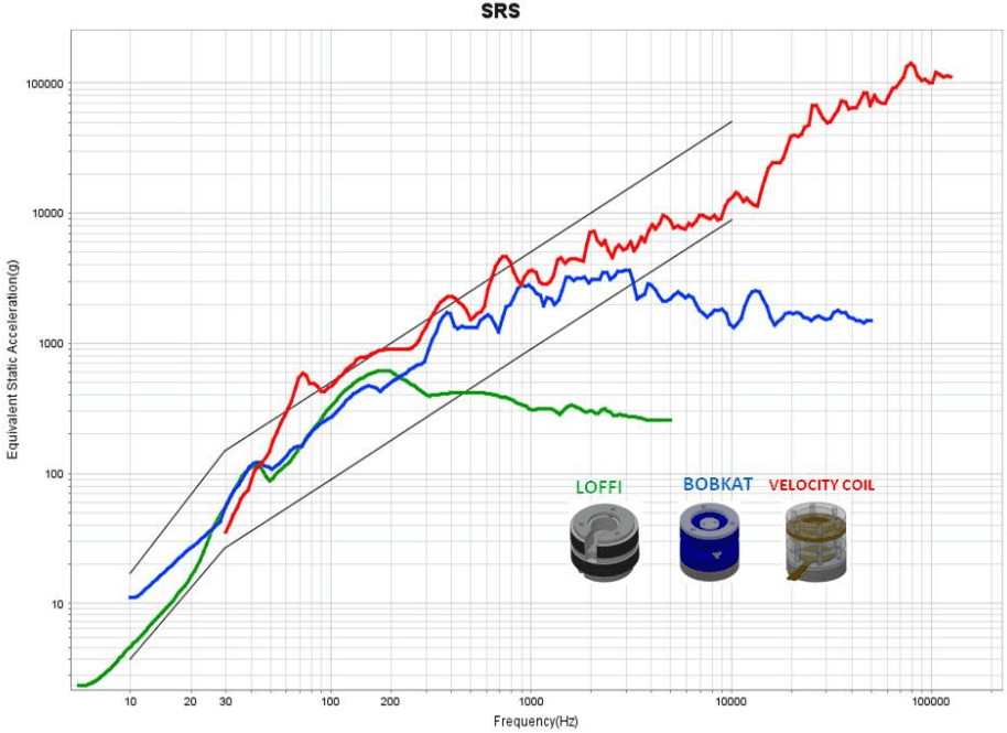
Figure description:
SRS
SRS
Legend
- LOFFI — color: green; symbol: solid line
- BOBKAT — color: blue; symbol: solid line
- VELOCITY COIL — color: red; symbol: solid line
Annotations
- Upper limit envelope (line - position: Defined by points (10, 17, (30, 150, and (10000, 50000))))
- Lower limit envelope (line - position: Defined by points (10, 4, (30, 25, and (10000, 9000))))
| Frequency(Hz) | LOFFI (g) | BOBKAT (g) | VELOCITY COIL (g) | Upper Limit (g) | Lower Limit (g) |
|---|---|---|---|---|---|
| 5 | 2.5 | null | null | null | null |
| 10 | 5 | 11 | null | 17 | 4 |
| 20 | 18 | 35 | null | 65 | 12 |
| 30 | 50 | 110 | 40 | 150 | 25 |
| 50 | 100 | 120 | 180 | 300 | 50 |
| 100 | 280 | 320 | 450 | 750 | 120 |
| 200 | 600 | 500 | 900 | 1800 | 280 |
| 500 | 420 | 1200 | 2500 | 5500 | 850 |
| 1000 | 320 | 3000 | 3500 | 12000 | 1800 |
| 2000 | 300 | 3200 | 7000 | 22000 | 3500 |
| 5000 | 260 | 2800 | 9000 | 50000 | 8500 |
| 10000 | null | 1500 | 14000 | 50000 | 9000 |
| 20000 | null | 1500 | 38000 | null | null |
| 30000 | null | 1800 | 70000 | null | null |
| 50000 | null | 1500 | 80000 | null | null |
| 70000 | null | null | 140000 | null | null |
| 100000 | null | null | 110000 | null | null |
| 150000 | null | null | 115000 | null | null |
Notes: The chart uses a logarithmic scale for both axes. The legend includes illustrative 3D models of the sensors. The black lines indicate boundary envelopes for the shock response spectra.
Figure 522.2-2. Shock Response Spectra from three different sensors needed to measure the entire spectrum
(5 Hz to 100,000 Hz) of a ballistic shock event.
Transducers used in ballistic shock applications must be evaluated in the ballistic shock environment (roughly 1 MHz, roughly 1 million g, described in paragraph 1.2.3 above). Both field testing (using high explosives) and laboratory testing (such as the TCU shock machine and laser vibrometer described in reference g) are required to qualify transducers for use in a ballistic shock environment.
4.4.2 Data Acquisition Instrumentation
4.4.2.1 Filtering and Frequency Response
The data recording instrumentation shall have flat frequency response to at least 100 kHz for at least one channel at each measurement location. Attenuation of 3 dB at 100 kHz is acceptable. The digitizing rate must be at least 2.5 times the filtering frequency. Note that when measurements of peak amplitude are used to qualify the shock level, a sample rate of at least 10 times the filtering frequency (1 million samples per second) is required. Additional, lower frequency measurement channels, at the same location may be used for lower frequency response measurements.
It is imperative that a responsibly designed system to reject aliasing is employed. Analog anti-alias filters must be in place before the digitizer. The selected anti-alias filtering must have an attenuation of 50 dB or greater, and a pass band flatness within one dB across the frequency bandwidth of interest for the measurement (see Figure 522.2-3). Subsequent resampling e.g., for purposes of decimation, must be in accordance with standard practices and consistent with the analog anti-alias configuration (e.g. digital anti-alias filters must be in place before subsequent decimations).
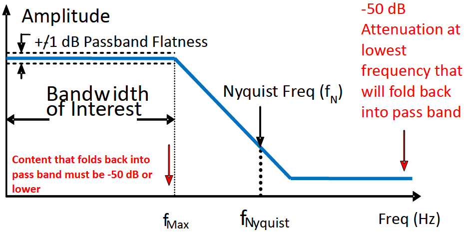
Figure description:
Amplitude vs Frequency Response
Low-pass Filter Characteristics
Annotations
- +/1 dB Passband Flatness (text_label - position: Passband region (0 to f_Max, y = 0 +/- 1 dB))
- Bandwidth of Interest (text_label - position: Horizontal interval [0, f_Max)
- Nyquist Freq (f_N (text_label - position: x = f_Nyquist, on the roll-off curve))
- Content that folds back into pass band must be -50 dB or lower (text_label - position: Indicated with a red arrow at f_Max)
- -50 dB Attenuation at lowest frequency that will fold back into pass band (text_label - position: Indicated with a red arrow pointing to the high frequency attenuation floor)
| Frequency (Hz) | Amplitude | Region / Key Point |
|---|---|---|
| 0 | 0 dB | Start of Passband |
| 0 to f_Max | 0 dB (+/- 1 dB) | Bandwidth of Interest |
| f_Max | 0 dB | End of Passband / Start of Roll-off |
| f_Nyquist | Intermediate | Nyquist Frequency (f_N) |
| High Frequencies | -50 dB | Stopband / Aliasing Suppression |
Notes: The chart illustrates the relationship between the bandwidth of interest (f_Max, the Nyquist frequency (f_Nyquist, and the required attenuation level (-50 dB to prevent significant aliasing in sampled systems.)))
Figure 522.2-3. Filter attenuation (conceptual, not filter specific).
The end to end alias rejection of the final discretized output must be shown to meet the requirements in Figure 522.2- 3. The anti-alias characteristics must provide attenuation of 50 dB or greater for frequencies that will fold back into the passband. Spectral data including SRS plots may only be presented for frequencies within the passband (between O and fmax). However, this restriction is not to constrain digital data validation procedures that require assessment of digitally acquired data to the Nyquist frequency (either for the initial ADC or subsequent resampled sequences).
Verification of alias rejection should start by establishing the dynamic range within the pass band in terms of the signal to noise ratio (SNR). The SNR = 2010g 10 (V FullScale/V Noisefloor) must be ≥60dB. Once sufficient SNR is verified, establishing the alias rejection characteristics may be determined using an input sine wave with a magnitude of 0.5 * full scale range and at the lowest frequency range that can impinge i.e., be aliased into fmax, and then confirming (using the IEEE 1057 sine wave test procedure or through inspection of the time domain data) that the alias rejection is sufficient at this frequency. If the 1 million sample/second digitizing rate is used, for example, then fNyquist = 500 kHz. Theory says that if a signal above the Nyquist Ratio is present, it will "fold over" into a frequency below the Nyquist ratio. The equation is:
, where
of "alias"
F = frequency of input signal
Fs = sample rate
n = integer number of sample rate (Fs) closest to input signal frequency (F)
Hence the lowest frequency range that can fold back into the 100 kHz passband is from 900 kHz to 1,100 kHz = 0.9 to 1.1 MHz.
It should be noted that Sigma Delta (SD) digitizers "oversample" internally at a rate several times faster than the output data rate. Analog anti-alias filtering for SD digitizers may be used at the Nyquist rate for the internal sample rate. For example, if a 1 million sample/second SD digitizer samples internally at 8 million samples/second, then the internal Nyquist frequency is 4 MHz, hence the analog anti-alias filter should remove content above 4 MHz that can fold back into the 100 kHz pass band (7.9 MHz to 8.1 MHz and similar bands that are higher in frequency). Figure 522.2-4 illustrates sampling frequencies, Nyquist frequencies, and frequency bands that can fold back into the bandwidth of interest for both conventional ("Successive Approximation") digitizers and over sampling digitizers, such as the Sigma Delta digitizer.
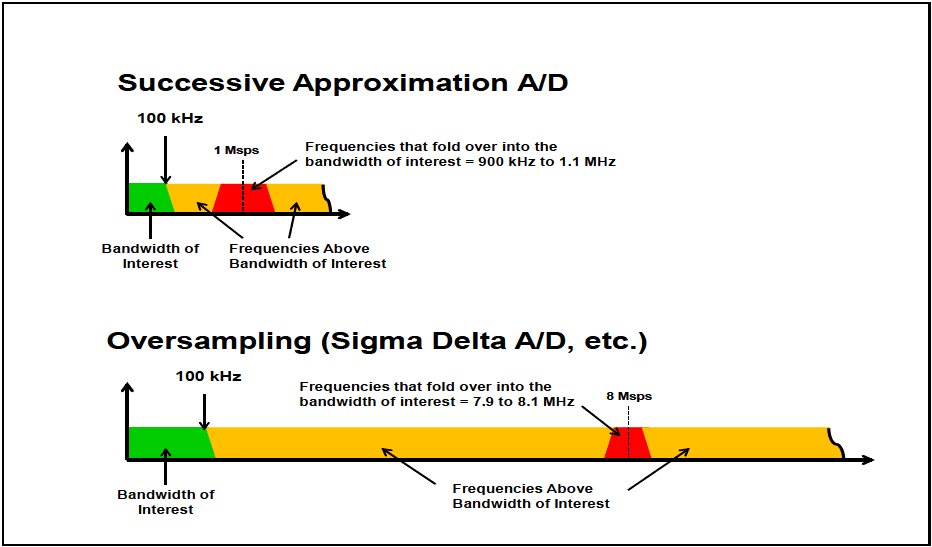
Figure description:
A/D Frequency Spectrum Comparisons
Successive Approximation A/D
Legend
- Bandwidth of Interest — color: Green; symbol: Filled region
- Frequencies Above Bandwidth of Interest — color: Yellow; symbol: Filled region
- Frequencies that fold over — color: Red; symbol: Filled region
Annotations
- 100 kHz (text_label - position: x = 100 kHz)
- 1 Msps (vertical_line - position: x = 1 Msps)
- Frequencies that fold over into the bandwidth of interest = 900 kHz to 1.1 MHz (shaded_area - position: x = 900 kHz to 1.1 MHz)
| Region | Frequency Range |
|---|---|
| Bandwidth of Interest | 0 to 100 kHz |
| Frequencies Above Bandwidth of Interest | > 100 kHz |
| Frequencies that fold over into the bandwidth of interest | 900 kHz to 1.1 MHz |
| Sampling Rate | 1 Msps |
Oversampling (Sigma Delta A/D, etc.
Legend
- Bandwidth of Interest — color: Green; symbol: Filled region
- Frequencies Above Bandwidth of Interest — color: Yellow; symbol: Filled region
- Frequencies that fold over — color: Red; symbol: Filled region
Annotations
- 100 kHz (text_label - position: x = 100 kHz)
- 8 Msps (vertical_line - position: x = 8 Msps)
- Frequencies that fold over into the bandwidth of interest = 7.9 to 8.1 MHz (shaded_area - position: x = 7.9 to 8.1 MHz)
| Region | Frequency Range |
|---|---|
| Bandwidth of Interest | 0 to 100 kHz |
| Frequencies Above Bandwidth of Interest | > 100 kHz |
| Frequencies that fold over into the bandwidth of interest | 7.9 to 8.1 MHz |
| Sampling Rate | 8 Msps |
Figure 522.2-4 Illustration of sampling rates and out of band "fold over" frequencies for data acquisition systems.
4.4.2.2 Slew Rate
To prevent distortion caused by spurious electrical noise, the data recording instrumentation shall be capable of recording a signal of one half full scale voltage in 1 microsecond without slew rate distortion. For example, if a system is capable of + 10 volts full scale = 20 volt peak-to-peak, then a slew rate of 10 volt/usecond is required.
4.4.2.3 Headroom
Undamped piezoelectric and Micro Electro-Mechanical System (MEMS) accelerometers are known to produce very high output signals at resonance (up to 100 times higher than the actual mechanical input). For Procedures I (BH&T), II (LSBSS), III (LWSM), and IV (Mechanical Shock Simulator), there is serious risk of significant “Out of Band Energy" being generated by undamped accelerometers. This high frequency "Out of Band Energy" is capable of causing distortion in the data recording electronics. Precautions must be taken (and documented) to insure that "Out of Band Energy" signals, produced by undamped accelerometers, do not distort "In Band” measurements, due to inadvertent clipping at various amplification stages of the analog signal conditioning. The following alternatives are examples of acceptable precautions:
-
a. Use of critically damped transducers (which do not produce significant “Out of Band Energy").
-
b. Use of long multi-conductor cables is not desirable, but is often unavoidable. Long cables can significantly attenuate the "Out of Band Energy" signals. If, for example, cable attenuation is shown to be -34 db (a factor of 50X), or more, at the resonant frequency of the undamped accelerometer, then the cable alone serves as acceptable protection from “Out of Band Energy”.
-
c. Use of an analog detector at each stage of amplification, to insure that no signal “clipping” occurs prior to filtering, serves as acceptable documentation as to where “Out of Band Energy” distortion did, or did not occur.
-
d. Setting the full scale recording range to a factor of roughly 25X above the expected signal level (i.e. a "Headroom" of 25X) serves as acceptable protection from internal clipping due to "Out of Band Energy". If the expected level was 2,000g, for example, the full scale range would be set to 50,000g. Hence a 50,000g "Out of Band Energy" signal could be accommodated without clipping. Unfortunately, the expected "In Band" signal level would only use 4% of the full scale capability of the recorder, compromising signal fidelity. Note that use of "Post Filter Gain" (gain applied after the anti-alias filter has removed the "Out of Band Energy"), reduces the amount of headroom required. In the previous example, the pre-filter gain would still be set to provide a range of 50,000g, but additional gain after the filter could amplify the signal before digitization, thereby increasing fidelity. The headroom of the post-filter gain would depend on knowledge of the expected in-band signal and fidelity requirements. For situations where the expected level is not well understood a post-filter gain overhead of 10X is recommended, or 20,000g in the example case.
4.5 Data Analysis
Detailed analysis procedures for evaluation of the problems peculiar to ballistic shock measurement have not been established. Many (but not all) of the techniques described in paragraph 6.1, reference f are appropriate.
4.6 Test Execution
4.6.1 Preparation for Test
4.6.1.1 Preliminary Steps
Prior to initiating any testing, review pretest information in the test plan to determine test details (e.g., procedures, test item configuration, ballistic shock levels, number of ballistic shocks):
- a. Choose the appropriate test procedure.
- b. If the ballistic shock is a calibrated test, determine the appropriate ballistic shock levels for the test prior to calibration.
- c. Ensure the ballistic shock signal conditioning and recording devices have adequate amplitude range and frequency bandwidth. It may be difficult to estimate a peak signal and arrange the instrumentation appropriately. In general there is no data recovery from a clipped signal. However, for over-ranged signal conditioning, it is usually possible to acquire meaningful results for a signal 20 dB above the noise floor of the measurement system. In some cases, redundant measurements may be appropriate - one measurement being over-ranged and one measurement ranged at the best estimate for the peak signal. The frequency bandwidth of most recording devices is usually readily available, but ensures that recording device input filtering does not limit the signal frequency bandwidth.
4.6.1.2 Pretest Checkout
All items require a pretest checkout at standard ambient conditions to provide baseline data. Conduct the checkout as follows:
Step 1 Conduct a complete visual examination of the test item with special attention to any micro electronic circuitry areas. Pay particular attention to its platform mounting configuration and potential stress wave transmission paths.
Step 2 Document the results.
Step 3 Where applicable, install the test item in its test fixture.
Step 4 Conduct an operational checkout in accordance with the approved test plan, along with simple tests for ensuring the measurement system is responding properly.
Step 5 Document the results for comparison with test data.
Step 6 If the test item operates satisfactorily, proceed to the first test. If not, resolve the problem and restart at Step 1.
MIL-STD-810H
METHOD 522.2
Step 7 Remove the test item and proceed with the calibration.
4.6.2 Procedures
The following procedures provide the basis for collecting the necessary information concerning the platform and test item undergoing ballistic shock. Since one of four or more ballistic shock devices may be employed, the instructions below must be consistent with the ballistic shock device selected.
4.6.2.1 Procedure I – BH&T
Step 1 Select the test conditions and mount the test item in a Ballistic Hull and Turret (BH&T), that may require ‘upweighting’ to achieve the proper dynamic response. (In general, there will be no calibration when actual hardware is used in this procedure). Select measurement techniques that have been validated in ballistic shock environments. See paragraph 6.1, reference g, for examples.
Step 2 Perform an operational check on the test item.
Step 3 Fire threat munitions at the BH&T and verify that the test item operates as required. Typically, make shock measurements at the mounting location (‘input shock’) and on the test item (‘test item response’).
Step 4 Record necessary data for comparison with pretest data.
Step 5 Photograph the test item as necessary to document damage.
Step 6 Perform an operational check on the test item. Record performance data. See paragraph 5 for analysis of results.
4.6.2.2 Procedure II – LSBSS
Step 1 Mount the test item to the LSBSS using the same mounting hardware as would be used in the actual armored vehicle. Select the orientation of the test item with the intent of producing the largest shock in the ‘worst case’ axis.
NOTE: A ‘dummy’ test item is typically mounted until measurements confirm that the proper explosive ‘recipe’ (i.e., combination of explosive weight, stand-off distance, and hydraulic displacement) has been determined to obtain the shock levels specified in Table 522.2-I and on Figure 522.2-1. Then mount an operational test item to the LSBSS.
Step 2 Fire the LSBSS and verify the test item is operating as required before, during, and after the shot. If the test item fails to operate as intended, follow the guidance in paragraph 4.3.2 for test item failure.
Step 3 Record initial data for comparison with post test data.
Step 4 Fire three test shots at the shock level specified in Table 522.2-I.
Step 5 Inspect the test item; photograph any noted damage, and record data for comparison with pretest data.
4.6.2.3 Procedure III – LWSM
Step 1 Modify the mounting for the anvil plate to restrict total travel (including dynamic plate deformation) to 15 mm (0.59 inch). Mount the test item to the LWSM using the same mounting hardware as would be used in an actual armored vehicle. Choose the orientation of the test item with the intent of producing the largest shock in the ‘worst case’ axis.
Step 2 Perform a pretest checkout and record data for comparison with post test data.
NOTE: Typically, make shock measurements at the ‘input’ location to ensure the low frequency shock levels specified in Table 522.2-I and in Figure 522.2-1 have been attained on the 1.5 m (5 foot) drop.
MIL-STD-810H
METHOD 522.2
- Step 3 Perform a 0.3 m (1 foot) hammer drop followed by an operational check; record data. If the test item fails to operate as intended, follow the guidance in paragraph 4.3.2 for test item failure. Otherwise, proceed to Step 4.
Step 4 Perform a 0.9 m (3 foot) hammer drop followed by an operational check; record data. If the test item fails to operate as intended, follow the guidance in paragraph 4.3.2 for test item failure. Otherwise, go to Step 5.
Step 5 Perform a 1.5 m (5 foot) hammer drop followed by an operational check; record data. If the test item fails to operate as intended, follow the guidance in paragraph 4.3.2 for test item failure.
Step 6 Repeat Step 5 two more times.
- Step 7 If the worst case axis is unknown (see paragraph 4.1c), repeat Steps 2-6 for each direction of each axis for a total of 18 five-foot hammer drops. See paragraph 5 for analysis of results.
4.6.2.4 Procedure IV – Mechanical Shock Simulator
- Step 1 Mount the test item to the Mechanical Shock Simulator using the same mounting hardware as would be used in the actual armored vehicle. Select the orientation of the test item with the intent of producing the largest shock in the ‘worst case’ axis.
- Step 2 Launch the mechanical shock simulator projectile and verify the test item is functioning as required before, during, and after the shot.
Step 3 Record initial data for comparison with post test data.
Step 4 Conduct three test shots at the shock level specified in Table 522.2-I.
- Step 5 If the worst case axis is unknown (see paragraph 4.1c), repeat Steps 2-6 for each direction of each axis, for a total of 18 projectile impacts.
- Step 6 Inspect the test item; photograph any noted damage, and record data for comparison with pretest data. Perform an operational check on the test item. Record performance data. See paragraph 5 for analysis of results.
4.6.2.5 Procedure V-MWSM
- Step 1 Modify the supports for the anvil table (by shimming the 4 table lifts) to restrict table total travel (including dynamic plate deformation) to 15 mm (0.59 inch).
- Step 2 Mount the test item to the MWSM using the same mounting hardware as would be used in an actual combat vehicle. Choose the orientation of the test item with the intent of producing the largest shock in the ‘worst case’ axis (see Step 7 below).
- Step 3 Perform a pretest checkout and record data for comparison with post test data.
NOTE: Typically, make shock measurements at the ‘input’ location to ensure that the low-frequency shock levels specified in Table 522.2-I and on Figure 522.2-1 have been attained on the ‘Group III’ drop (from MIL-S-901).
- Step 4 Perform a ‘Group I height’ hammer drop followed by an operational check; record data. If the test item fails to operate as intended, follow the guidance in paragraph 4.3.2 for test item failure.
- Step 5 Perform a ‘Group III height’ hammer drop followed by an operational check; record data.
Step 6 Repeat Step 5 two more times.
- Step 7 If the worst case axis is unknown (see paragraph 4.1c), repeat Steps 2-6 for each direction of each axis for a total of 18 hammer drops at the Group III height.
MIL-STD-810H
METHOD 522.2
4.6.2.6 Procedure VI – Drop Table
Step 1 Calculate the expected response of a shock mounted test item (or measurements from field tests may be used) and calculate a shock response spectra (SRS). Choose a half-sine acceleration pulse whose SRS ‘envelopes’ the expected response of the shock mounted item. Note that this approach typically results in an overtest at the lowest frequencies.
Step 2 Hard mount the test item to the drop table.
Step 3 Conduct an operational check and record data for comparison with post test data. If the test item operates satisfactorily, proceed to Step 4. If not, resolve the problems and repeat this step.
Step 4 Test using the appropriate half-sine acceleration pulse three times in each direction of all three axes (18 drops).
Step 5 Conduct a performance check and record data for comparison with pretest data. See paragraph 5 for analysis of results.