| Paragraph | Page | |
|---|---|---|
| 4.5.2 | PROCEDURE SPECIFIC. | 17 |
| 4.5.2.1 | PROCEDURE I-SESA REPLICATION OF A FIELD MEASURED MATERIEL TIME TRACE INPUT/RESPONSE. | 17 |
| 4.5.2.2 | PROCEDURE II-SESA REPLICATION OF AN ANALYTICALLY SPECIFIED MATERIEL TIME TRACE INPUT/RESPONSE | 18 |
| 4.5.3 | DATA ANALYSIS | 18 |
| 5. | ANALYSIS OF RESULTS.. | 18 |
| 5.1 | PHYSICS OF FAILURE.. | 18 |
| 5.2 | QUALIFICATION TESTS. | 18 |
| 5.3 | OTHER TESTS | 19 |
| 6. | REFERENCE/RELATED DOCUMENTS. | 19 |
| 6.1 | REFERENCED DOCUMENTS | 19 |
| 6.2 | RELATED DOCUMENTS.. | 19 |
FIGURES
| FIGURE 525.2-1. | BASIC TWR TEST MODES AS RELATED TO TIME TRACE SCALING | 4 |
| FIGURE 525.2-2. | BASIC TWR TEST SIMULATION COMBINATIONS | 6 |
METHOD 525.2, ANNEX A SESA POST-TEST ANALYSIS ILLUSTRATION FOR TEST TOLERANCE ASSESSMENT
| 1. | PURPOSE | A-1 |
| 2. | GENERAL PHILOSOPHY FOR TWR TESTING | A-1 |
| 3. | DESCRIPTION OF REFERENCE TIME TRACE | A-1 |
| 4. | TIME TRACE PRE-PROCESSING | A-2 |
| 4.1 | INTRODUCTION | A-2 |
| 4.2 | FREQUENCY BAND LIMITING | A-4 |
| 4.3 | TIME TRACE CORRELATION | A-5 |
| 4.4 | TIME TRACE SEGMENT IDENTIFICATION | A-6 |
| 5. | POST-TEST PROCESSING FOR TPP | A-9 |
| 6. | TPP TRANSIENT VIBRATION | A-10 |
| 7. | TPP STATIONARY VIBRATION | A-13 |
| 8. | TPP SHOCK | A-18 |
| 9. | POST-TEST PROCESSING FOR STA | A-22 |
MIL-STD-810H METHOD
525.2 CONTENTS - Continued Paragraph
| ANNEX A FIGURES | ||
| FIGURE 525.2A-1. | FIELD MEASURED ACCELERATION REFERENCE TIME TRACE | A-2 |
| FIGURE 525.2A-2A. | EXCITER HEAD (H) (REFERENCE/CONTROL TIME TRACES PRIOR TO POST-TEST PREPROCESSING). | .A-3 |
| FIGURE 525.2A-2B. | EXCITER SLIP TABLE (S) (REFERENCE/CONTROL TIME TRACES PRIOR TO POST-TEST PREPROCESSING).. | A-3 |
| FIGURE 525.2A-3. | REFERENCE/CONTROL TIME TRACE PERIODOGRAMS FOR FREQUENCY BAND-LIMITING THROUGH FFT WINDOW FILTERING | .A-5 |
| FIGURE 525.2A-4. | CROSS-COVARIANCE FUNCTION ESTIMATES BETWEEN REFERENCE AND CONTROL TIME TRACES | ..A-6 |
| FIGURE 525.2A-5. | TIME TRACE SEGMENT IDENTIFICATION FROM PREVIOUSLY TRUNCATED REFERENCE TIME TRACES | .A-7 |
| FIGURE 525.2A-6. | TRANSIENT VIBRATION REFERENCE TIME TRACE SEGMENT. | A-7 |
| FIGURE 525.2A-7. | STATIONARY RANDOM VIBRATION REFERENCE TIME TRACE SEGMENT. | .A-8 |
| FIGURE 525.2A-8. | SHOCK REFERENCE TIME TRACE SEGMENT | .A-8 |
| FIGURE 525.2A-9. | PLOTS OF OVERALL DIFFERENCE TIME TRACE WITH ROOT-MEAN-SQUARE.. | .A-9 |
| FIGURE 525.2A-9A. | DIFFERENCE EXCITER (H). | .A-9 |
| FIGURE 525.2A-9B. | DIFFERENCE EXCITER (S) | .A-9 |
| FIGURE 525.2A-9C. | TIME TRACE OF DIFFERENCE OF THE DIFFERENCES ((S) - (H)). | .A-9 |
| FIGURE 525.2A-10. | TRANSIENT VIBRATION TIME TRACES -R, C, AND S | .A-10 |
| FIGURE 525.2A-11. | R VERSUS C CROSS-PLOT | A-11 |
| FIGURE 525.2A-12. | TRANSIENT VIBRATION Q-Q PLOT FOR S VERSUS GAUSSIAN | A-11 |
| FIGURE 525.2A-13. | COMPOSITE ROOT-MEAN-SQUARE ENVELOPE ESTIMATES FOR R AND C | A-12 |
| FIGURE 525.2A-14. | COMPOSITE NORMALIZED ASD ESTIMATES FOR R AND C | .A-12 |
| FIGURE 525.2A-15. | STATIONARY VIBRATION TIME TRACES - R, C, AND S | A-13 |
| FIGURE 525.2A-16. | STATIONARY VIBRATION PROBABILITY DENSITY FUNCTION ESTIMATES | A-14 |
| FIGURE 525.2A-17. | STATIONARY VIBRATION Q-Q PLOT FOR S VERSUS GAUSSIAN | .A-14 |
| FIGURE 525.2A-18A. | FOT ERROR ASSESSMENT - 10% REA ERROR FRACTION-OF-TIME (FOT) | A-15 |
| FIGURE 525.2A-18B. | FOT ERROR ASSESSMENT -5% REA FOT ERROR BOUNDS | .A-16 |
| FIGURE 525.2A-18c. | FOT ERROR ASSESSMENT - ONE SIDED 10% REA FOT ERROR BOUNDS | .A-16 |
| FIGURE 525.2A-19A. | COMPOSITE ASD ESTIMATES FOR R AND C.. | .A-17 |
| FIGURE 525.2A-19B. | ASD ESTIMATE FOR S | .A-17 |
| FIGURE 525.2A-20. | SHOCK TIME TRACES-R, C, AND S. | .A-18 |
| FIGURE 525.2A-21. | R VERSUS C CROSS-PLOT | .A-19 |
| FIGURE 525.2A-22. | SHOCK Q-Q PLOT FOR S VERSUS GAUSSIAN | .A-19 |
| FIGURE 525.2A-23A. | COMPOSITE PSEUDO-VELOCITY MAXIMAX PSEUDO-VELOCITY SRS FOR R AND C. | .A-20 |
| FIGURE 525.2A-23B. | COMPOSITE PSEUDO-VELOCITY MAXIMAX ACCELERATION SRS FOR R AND C. | A-20 |
| FIGURE 525.2A-24. | ESD ESTIMATES FOR R AND C. | A-21 |
| FIGURE 525.2A-25. | ESD ESTIMATE FOR S | .A-21 |
| FIGURE 525.2A-26. | SHORT-TIME AVERAGING FOR DIFFERENCE MEAN | .A-22 |
| FIGURE 525.2A-27. | SHORT-TIME AVERAGING FOR DIFFERENCE ROOT-MEAN-SQUARE. | .A-23 |
Page METHOD 525.2, ANNEX B SUMMARY OF POST-TEST ANALYSIS PROCESSING PROCEDURES AND TEST TOLERANCE SPECIFICATION
| 1. | INTRODUCTION | B-1 |
| 2. | TERMINOLOGY | B-1 |
| 3. | REPLICATION ERROR (TEST TOLERANCE) ASSESSMENT EXPRESSIONS | B-2 |
| 4. | REPLICATION ERROR TOLERANCE SPECIFICATION | B-9 |
MIL-STD-810H METHOD
525.2 CONTENTS - Continued
| Paragraph | Page |
|---|---|
| ANNEX B TABLE | |
| TABLE 525.2B-I. SUMMARY OF ERROR ASSESSMENT EXPRESSIONS | B-3 |
MIL-STD-810H
METHOD
525.2 TIME WAVEFORM REPLICATION
NOTE: Tailoring is required. Select methods, procedures, and parameter levels based on the tailoring process described in Part One, paragraph 4.2.2, and Annex C. Apply the general guidelines for laboratory test methods described in Part One, paragraph 5 of this Standard.
525.2 ANNEX A
525.2 ANNEX A
confidence (dependent upon the accuracy of the covariance function estimate). Figure 525.2A-4 provides a biased cross-covariance function estimate between the band-limited reference and control time traces.
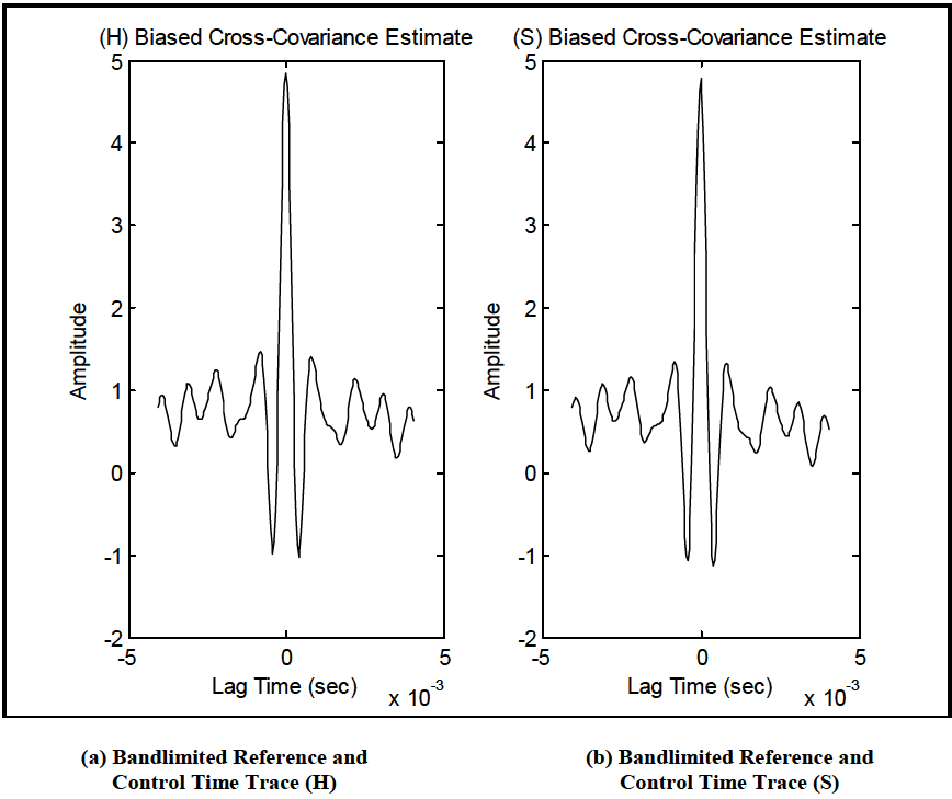
Figure description:
Bandlimited Reference and Control Time Traces
(H Biased Cross-Covariance Estimate
| Lag Time (sec x 10^-3) | Amplitude |
|---|---|
| -4.0 | 0.8 |
| -3.5 | 0.4 |
| -3.0 | 1.1 |
| -2.5 | 0.7 |
| -2.0 | 1.2 |
| -1.5 | 0.4 |
| -1.0 | 1.5 |
| -0.5 | -1.0 |
| 0.0 | 4.8 |
| 0.5 | -1.0 |
| 1.0 | 1.4 |
| 1.5 | 0.5 |
| 2.0 | 1.1 |
| 2.5 | 0.4 |
| 3.0 | 1.1 |
| 3.5 | 0.2 |
| 4.0 | 0.8 |
(S Biased Cross-Covariance Estimate
| Lag Time (sec x 10^-3) | Amplitude |
|---|---|
| -4.0 | 0.9 |
| -3.5 | 0.3 |
| -3.0 | 1.1 |
| -2.5 | 0.6 |
| -2.0 | 1.2 |
| -1.5 | 0.4 |
| -1.0 | 1.3 |
| -0.5 | -1.1 |
| 0.0 | 4.8 |
| 0.5 | -1.1 |
| 1.0 | 1.3 |
| 1.5 | 0.4 |
| 2.0 | 1.0 |
| 2.5 | 0.3 |
| 3.0 | 1.0 |
| 3.5 | 0.1 |
| 4.0 | 0.7 |
Figure 525.2A-4. Cross-covariance function estimates between reference and control time traces.
By examining the cross-correlation estimate region near a lag of zero seconds, it is apparent that the reference and control time traces are in phase, and no shifting of one time trace relative to the other is necessary.
525.2 ANNEX A
525.2 ANNEX A
Figure 525.2A-13 provides an overlay of envelopes of r and c in terms of root-mean-square g's for a short-time averaging increment of 0.1 seconds (STA assessment). If the product model can be assumed, the differences in root- mean-square envelope levels are a maximum of 2 percent.
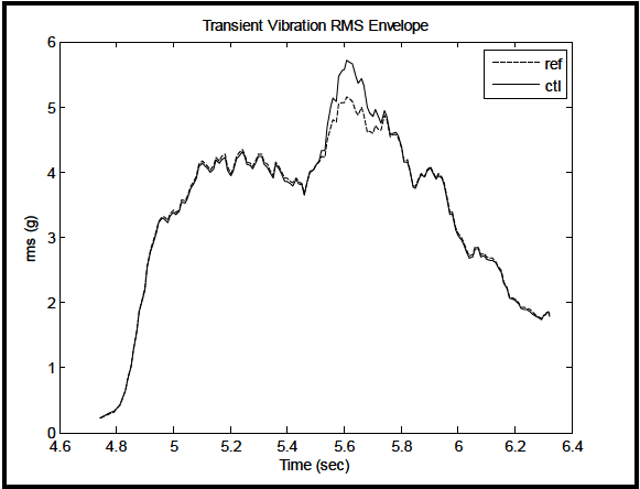
Figure description:
Transient Vibration RMS Envelope
Transient Vibration RMS Envelope
Legend
- ref — color: black; symbol: Dashed line
- ctl — color: black; symbol: Solid line
| Time (sec) | ref rms (g) | ctl rms (g) |
|---|---|---|
| 4.75 | 0.25 | 0.25 |
| 4.80 | 0.40 | 0.40 |
| 4.85 | 0.90 | 0.90 |
| 4.90 | 1.90 | 1.90 |
| 4.95 | 3.10 | 3.10 |
| 5.00 | 3.35 | 3.35 |
| 5.05 | 3.65 | 3.65 |
| 5.10 | 4.15 | 4.15 |
| 5.15 | 4.30 | 4.30 |
| 5.20 | 4.10 | 4.10 |
| 5.25 | 4.35 | 4.35 |
| 5.30 | 4.15 | 4.15 |
| 5.35 | 3.90 | 3.90 |
| 5.40 | 3.85 | 3.85 |
| 5.45 | 3.75 | 3.75 |
| 5.50 | 4.10 | 4.10 |
| 5.55 | 4.60 | 4.70 |
| 5.60 | 5.10 | 5.65 |
| 5.65 | 5.00 | 5.45 |
| 5.70 | 4.70 | 4.85 |
| 5.75 | 4.75 | 4.80 |
| 5.80 | 4.20 | 4.20 |
| 5.85 | 3.80 | 3.80 |
| 5.90 | 4.05 | 4.05 |
| 5.95 | 3.75 | 3.75 |
| 6.00 | 3.10 | 3.10 |
| 6.05 | 2.75 | 2.75 |
| 6.10 | 2.70 | 2.70 |
| 6.15 | 2.45 | 2.45 |
| 6.20 | 2.00 | 2.00 |
| 6.25 | 1.85 | 1.85 |
| 6.30 | 1.80 | 1.80 |
Notes: The chart shows the root mean square (RMS vibration envelope over time, comparing a reference ('ref' signal to a controlled ('ctl' signal. The signals are largely identical except for a period between approximately 5.5 and 5.7 seconds where the 'ctl' signal exhibits a higher peak.)))
Figure 525.2A-13. Composite root-mean-square envelope estimates for r and c.
Figure 525.2A-14 provides a composite of normalized ASD estimates for r and c. The estimates were determined by one-sixth octave band frequency averaging. The normalized ASD estimates differ by less than 2 dB.
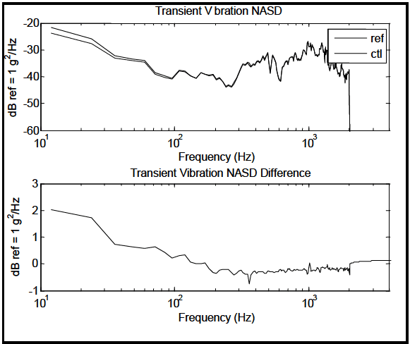
Figure description:
Transient Vibration NASD Analysis
Transient Vibration NASD
Legend
- ref — color: gray; symbol: Solid line
- ctl — color: black; symbol: Solid line
| Frequency (Hz) | ref (dB ref = 1 g²/Hz) | ctl (dB ref = 1 g²/Hz) |
|---|---|---|
| 11.2 | -21.8 | -23.8 |
| 15.8 | -23.5 | -25.2 |
| 20.0 | -24.5 | -26.3 |
| 25.1 | -25.8 | -27.5 |
| 31.6 | -29.0 | -30.5 |
| 39.8 | -32.5 | -33.2 |
| 50.1 | -33.5 | -34.0 |
| 63.1 | -34.0 | -34.6 |
| 79.4 | -39.0 | -39.6 |
| 100.0 | -37.5 | -37.7 |
| 125.9 | -40.5 | -40.5 |
| 158.5 | -38.5 | -38.5 |
| 199.5 | -39.8 | -40.0 |
| 251.2 | -43.0 | -43.0 |
| 316.2 | -44.2 | -44.0 |
| 398.1 | -34.8 | -35.2 |
| 501.2 | -35.0 | -35.0 |
| 631.0 | -32.0 | -32.3 |
| 794.3 | -34.5 | -34.8 |
| 1000.0 | -27.2 | -27.5 |
| 1258.9 | -29.0 | -29.0 |
| 1584.9 | -37.0 | -37.0 |
| 1995.3 | -39.5 | -39.8 |
| 2100.0 | -60.0 | -60.0 |
Transient Vibration NASD Difference
| Frequency (Hz) | Difference (dB ref = 1 g²/Hz) |
|---|---|
| 11.2 | 2.0 |
| 15.8 | 1.9 |
| 20.0 | 1.8 |
| 25.1 | 1.7 |
| 31.6 | 1.2 |
| 39.8 | 0.7 |
| 50.1 | 0.6 |
| 63.1 | 0.5 |
| 79.4 | 0.6 |
| 100.0 | 0.2 |
| 125.9 | 0.3 |
| 158.5 | 0.0 |
| 199.5 | -0.3 |
| 251.2 | -0.2 |
| 316.2 | -0.3 |
| 398.1 | -0.4 |
| 501.2 | -0.3 |
| 631.0 | -0.3 |
| 794.3 | -0.3 |
| 1000.0 | -0.3 |
| 1258.9 | -0.2 |
| 1584.9 | -0.2 |
| 1995.3 | 0.0 |
| 2100.0 | 0.1 |
Notes: The top plot shows the Power Spectral Density (PSD for reference (ref and control (ctl signals. The bottom plot shows the difference (ref - ctl in dB. The x-axis for both plots is logarithmic frequency.))))
Figure 525.2A-14. Composite normalized ASD estimates for r and c.
From the above statistics, it can be concluded that no valid distinction can be made between r and c under the product model assumption, even though the non-Gaussian distribution of errors is difficult to interpret. It would appear that tolerance for this particular segment could be established as less than 0.2 grms amplitude for 90 percent of the time
MIL-STD-810H METHOD
525.2 ANNEX A
trace envelope, and 2 dB for the normalized ASD estimates, based on the information in Figures 525.2A-13 and 525.2A-14. This concludes replication error processing and tolerance specification for the transient vibration sub- event.
525.2 ANNEX A
Annex B defines the FOT distribution for difference time trace assessment. This assessment empirically defines the
fraction of time the error lies outside (or inside) given error amplitude bounds. This assessment is mathematically equivalent to a probability density (or distribution) assessment but more transparent and easier to interpret for an allowable error tolerance specification. Since TWR is time based, an allowable error of x-percent of the time the error amplitude may exceed y-percent of the root-energy-amplitude level (REA) of the deterministic reference time trace is easily visualized. Figures 525.2A-18a,b,c display the time-varying error in g’s for the stationary segment along with the REA percentage error plotted against the FOT quantiles. For the example under consideration the REA for the reference is 1.85 g-rms. Both two-sided and one-sided analyses are considered. The FOT ranges from 0.0 to 1.0 over approximately plus and minus 10% of the REA. Figure 525.2A-18a displays FOT quantiles for 10% to 10% REA error percentage. Figure 525.2A-18b displays the REA random error -5% to 5% for FOT quantiles from approximately 0.1 to 0.9 and Figure 525.2A-18c considers one-sided error for 10% REA error percentage and the 0.90 FOT quantile. A two-sided tolerance specification might, for example, require not more than 10% (0.10 FOT quantile) of test time to lie outside the REA amplitude percentage bounds of -5% and 5%. Tolerance is in terms of what percentage of time is the error allowed to be larger than a certain percentage of REA as a reference amplitude.
In Figure 525.2A-19, a composite of the ASD estimates for r and c is provided. The ASD estimates between r and c are essentially equivalent. For time trace s, there is non-flat spectrum that normally would not be present if the replication error were of a strong Gaussian character, i.e., s was band-limited white noise. The processing parameters are an analysis bandwidth of 5 Hz applying a Hamming window with 50 percent overlap.
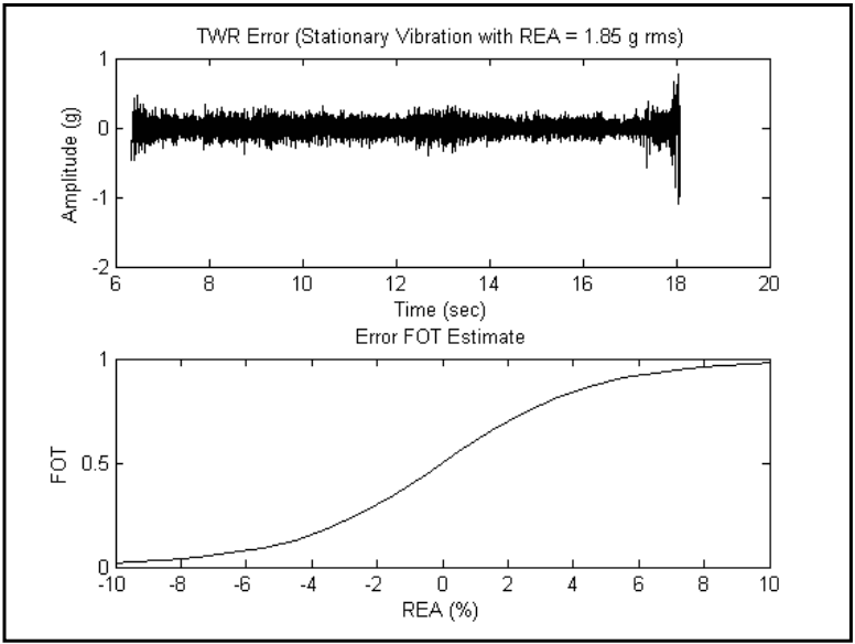
Figure description:
TWR Error (Stationary Vibration with REA = 1.85 g rms
| Time (sec) | Amplitude (g) |
|---|---|
| 6.30 | -0.15 |
| 6.45 | 0.45 |
| 6.50 | -0.40 |
| 7.00 | 0.25 |
| 8.00 | -0.20 |
| 9.00 | 0.30 |
| 10.00 | -0.25 |
| 11.00 | 0.20 |
| 12.00 | -0.30 |
| 13.00 | 0.35 |
| 14.00 | -0.20 |
| 15.00 | 0.25 |
| 16.00 | -0.25 |
| 17.00 | 0.30 |
| 17.40 | -0.60 |
| 17.60 | 0.40 |
| 17.80 | -0.85 |
| 18.00 | 0.75 |
| 18.10 | -1.10 |
| 18.15 | 0.80 |
Error FOT Estimate
| REA (%) | FOT |
|---|---|
| -10 | 0.02 |
| -8 | 0.04 |
| -6 | 0.08 |
| -4 | 0.15 |
| -2 | 0.30 |
| 0 | 0.50 |
| 2 | 0.70 |
| 4 | 0.85 |
| 6 | 0.92 |
| 8 | 0.96 |
| 10 | 0.98 |
Notes: The first chart shows a high-frequency noise signal with a significant increase in variance (instability just before termination at approximately 18 seconds. The second chart depicts a sigmoid cumulative distribution function for the FOT estimate against REA (%.))
Figure 525.2A-18a. FOT Error Assessment – 10% REA Error Fraction-of-Time (FOT)
MIL-STD-810H METHOD 525.2 ANNEX A
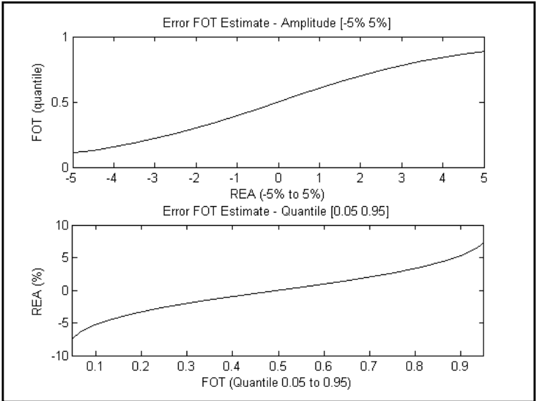
Figure description:
Error FOT Estimate Analysis
Error FOT Estimate - Amplitude [-5% 5%
| REA (-5% to 5%) | FOT (quantile) |
|---|---|
| -5 | 0.12 |
| -4 | 0.17 |
| -3 | 0.24 |
| -2 | 0.32 |
| -1 | 0.41 |
| 0 | 0.50 |
| 1 | 0.60 |
| 2 | 0.70 |
| 3 | 0.78 |
| 4 | 0.84 |
| 5 | 0.88 |
Error FOT Estimate - Quantile [0.05 0.95
| FOT (Quantile 0.05 to 0.95) | REA (%) |
|---|---|
| 0.05 | -7.5 |
| 0.1 | -5.8 |
| 0.2 | -3.8 |
| 0.3 | -2.4 |
| 0.4 | -1.2 |
| 0.5 | 0.0 |
| 0.6 | 1.2 |
| 0.7 | 2.4 |
| 0.8 | 3.8 |
| 0.9 | 5.8 |
| 0.95 | 7.5 |
Notes: The two charts represent the relationship between Relative Error Amplitude (REA and the Fraction of Time (FOT quantile. The top chart shows the cumulative distribution function (CDF and the bottom chart shows its inverse, the quantile function.)))
Figure 525.2A-18b FOT Error Assessment - 5% REA FOT Error Bounds
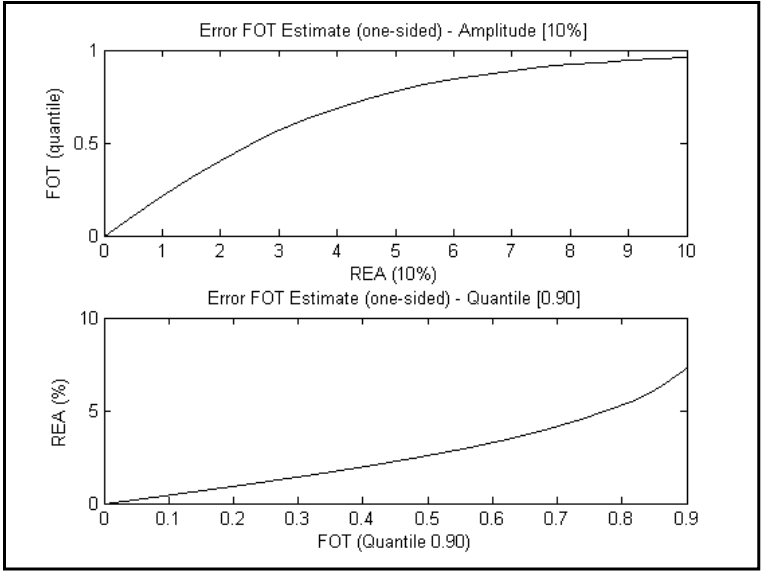
Figure description:
Error FOT Estimate (one-sided - Amplitude [10%
| REA (10%) | FOT (quantile) |
|---|---|
| 0 | 0.00 |
| 1 | 0.22 |
| 2 | 0.41 |
| 3 | 0.56 |
| 4 | 0.68 |
| 5 | 0.78 |
| 6 | 0.85 |
| 7 | 0.91 |
| 8 | 0.94 |
| 9 | 0.96 |
| 10 | 0.97 |
Error FOT Estimate (one-sided - Quantile [0.90
| FOT (Quantile 0.90) | REA (%) |
|---|---|
| 0.0 | 0.0 |
| 0.1 | 0.5 |
| 0.2 | 1.1 |
| 0.3 | 1.6 |
| 0.4 | 2.2 |
| 0.5 | 3.0 |
| 0.6 | 3.8 |
| 0.7 | 4.8 |
| 0.8 | 6.0 |
| 0.9 | 7.5 |
Figure 525.2A-18c FOT Error Assessment - One-sided 10% REA FOT Error Bounds
MIL-STD-810H METHOD 525.2 ANNEX A
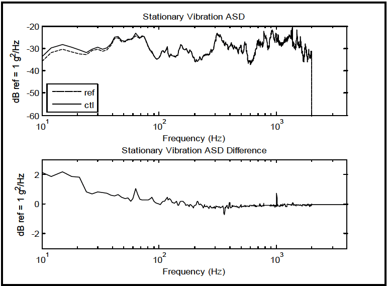
Figure description:
Stationary Vibration Analysis
Stationary Vibration ASD
Legend
- ref — color: black; symbol: Dashed line
- ctl — color: black; symbol: Solid line
| Frequency (Hz) | ref (dB ref = 1 g^2/Hz) | ctl (dB ref = 1 g^2/Hz) |
|---|---|---|
| 10 | -35.5 | -33.4 |
| 12 | -31.0 | -29.0 |
| 15 | -30.4 | -28.2 |
| 20 | -32.5 | -30.7 |
| 25 | -31.8 | -31.0 |
| 30 | -31.5 | -30.7 |
| 40 | -30.1 | -29.4 |
| 50 | -25.2 | -24.8 |
| 60 | -26.8 | -26.5 |
| 70 | -24.2 | -23.1 |
| 80 | -24.8 | -24.5 |
| 100 | -34.8 | -34.3 |
| 150 | -28.2 | -28.1 |
| 200 | -34.1 | -34.2 |
| 300 | -23.0 | -23.2 |
| 400 | -30.1 | -30.1 |
| 500 | -32.5 | -32.6 |
| 750 | -26.2 | -26.3 |
| 1000 | -22.5 | -21.7 |
| 1500 | -28.1 | -28.1 |
| 2000 | -32.0 | -32.0 |
| 2100 | -60.0 | -60.0 |
Stationary Vibration ASD Difference
| Frequency (Hz) | Difference (dB ref = 1 g^2/Hz) |
|---|---|
| 10 | 2.1 |
| 12 | 2.0 |
| 15 | 2.2 |
| 20 | 1.8 |
| 25 | 0.8 |
| 30 | 0.8 |
| 40 | 0.7 |
| 50 | 0.4 |
| 60 | 0.3 |
| 70 | 1.1 |
| 80 | 0.3 |
| 100 | 0.5 |
| 150 | 0.1 |
| 200 | -0.1 |
| 300 | -0.2 |
| 400 | 0.0 |
| 500 | -0.1 |
| 1000 | 0.8 |
| 1500 | 0.0 |
| 2000 | 0.0 |
Notes: The frequency axis is logarithmic. The lower chart represents the difference between the control (ctl and reference (ref signals shown in the upper chart.))
Figure 525.2A-19a. Composite ASD estimates for r and c.
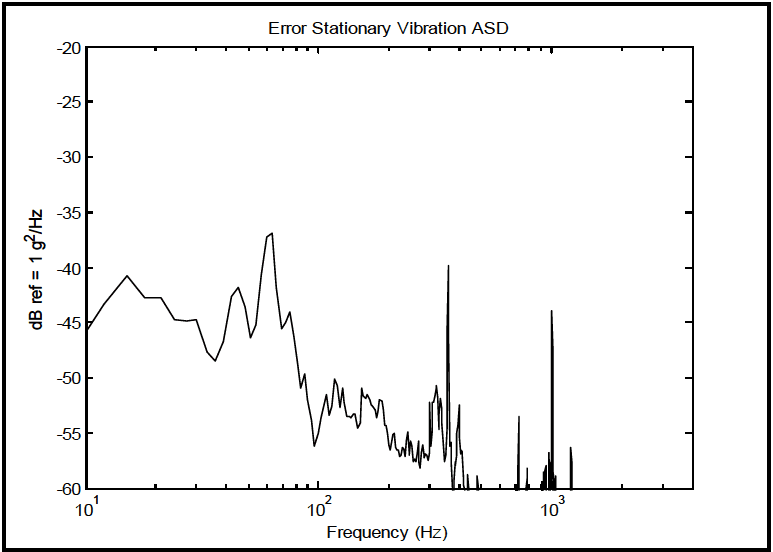
Figure description:
Error Stationary Vibration ASD
Error Stationary Vibration ASD
| Frequency (Hz) | dB ref = 1 g²/Hz |
|---|---|
| 10 | -46.0 |
| 15 | -40.7 |
| 20 | -42.6 |
| 25 | -42.6 |
| 30 | -44.7 |
| 35 | -47.6 |
| 40 | -48.5 |
| 45 | -46.5 |
| 50 | -41.7 |
| 60 | -46.2 |
| 70 | -37.2 |
| 75 | -36.9 |
| 85 | -45.4 |
| 95 | -43.9 |
| 100 | -56.1 |
| 112 | -51.5 |
| 125 | -53.3 |
| 140 | -50.1 |
| 160 | -53.4 |
| 180 | -50.9 |
| 200 | -53.4 |
| 220 | -51.9 |
| 250 | -56.5 |
| 300 | -56.4 |
| 350 | -50.7 |
| 400 | -39.7 |
| 450 | -58.5 |
| 500 | -59.5 |
| 600 | -59.9 |
| 700 | -53.5 |
| 850 | -58.2 |
| 1000 | -43.7 |
| 1100 | -56.4 |
| 1200 | -60.0 |
Notes: The x-axis is on a logarithmic scale, while the y-axis is on a linear scale representing values in decibels (dB.)
|
Figure 525.2A-19b. ASD estimate for s.
From the above statistics, it might be concluded that no valid distinction can be made between r and c under the stationary model assumption even though the non-Gaussian distribution of error s is difficult to interpret. It would
MIL-STD-810H METHOD
525.2 ANNEX A
|
appear that tolerances for this particular segment could be established as maximum 2 dB for the ASD estimates, based on the information in Figure 525.2A-19. This concludes replication error processing and tolerance development for the stationary vibration sub-event.
|
525.2 ANNEX A
A common way of comparing shock information is through the SRS, in particular the recommended pseudo-velocity SRS estimate (Method 516.8). For the r and c time traces, a composite overlay of the pseudo-velocity SRS estimates for both shocks is useful. Figure 525.2A-23 provides this comparison in addition to a maximax acceleration SRS comparison. Since the SRS is an integration/smoothing process, it is expected that the reference and control information will be highly correlated when viewed in an SRS format. For these figures no wavelet correction was attempted for low frequency correction since such a correction applied individually may lead to a less transparent comparison.
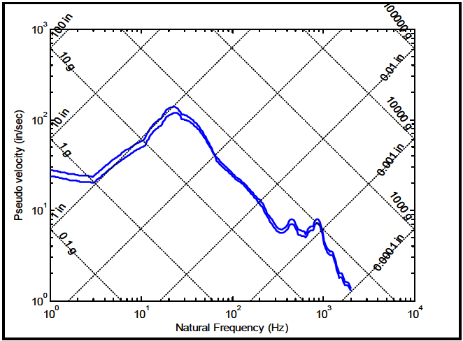
Figure description:
Shock Response Spectrum (Pseudo velocity vs. Natural Frequency
Shock Response Spectrum
Legend
- Upper Bound — color: blue; symbol: Solid line
- Lower Bound — color: blue; symbol: Solid line
Annotations
- 100 in (diagonal_line - position: Displacement constant line (downward slope))
- 10 in (diagonal_line - position: Displacement constant line (downward slope))
- 1 in (diagonal_line - position: Displacement constant line (downward slope))
- 0.1 in (diagonal_line - position: Displacement constant line (downward slope))
- 0.01 in (diagonal_line - position: Displacement constant line (downward slope))
- 0.001 in (diagonal_line - position: Displacement constant line (downward slope))
- 0.0001 in (diagonal_line - position: Displacement constant line (downward slope))
- 0.1 g (diagonal_line - position: Acceleration constant line (upward slope))
- 1 g (diagonal_line - position: Acceleration constant line (upward slope))
- 10 g (diagonal_line - position: Acceleration constant line (upward slope))
- 100 g (diagonal_line - position: Acceleration constant line (upward slope))
- 1000 g (diagonal_line - position: Acceleration constant line (upward slope))
- 10000 g (diagonal_line - position: Acceleration constant line (upward slope))
- 100000 g (diagonal_line - position: Acceleration constant line (upward slope))
| Natural Frequency (Hz) | Pseudo Velocity - Upper Bound (in/sec) | Pseudo Velocity - Lower Bound (in/sec) |
|---|---|---|
| 1.0 | 27.0 | 23.0 |
| 1.5 | 24.5 | 21.0 |
| 2.0 | 23.0 | 20.0 |
| 2.5 | 22.0 | 19.5 |
| 3.0 | 25.0 | 21.0 |
| 4.0 | 29.0 | 25.0 |
| 5.0 | 33.0 | 29.0 |
| 7.0 | 42.0 | 36.0 |
| 10.0 | 58.0 | 50.0 |
| 15.0 | 100.0 | 85.0 |
| 20.0 | 130.0 | 110.0 |
| 22.0 | 140.0 | 120.0 |
| 25.0 | 135.0 | 115.0 |
| 30.0 | 125.0 | 110.0 |
| 40.0 | 95.0 | 85.0 |
| 50.0 | 75.0 | 70.0 |
| 60.0 | 50.0 | 48.0 |
| 80.0 | 35.0 | 33.0 |
| 100.0 | 28.0 | 26.0 |
| 150.0 | 18.0 | 17.0 |
| 200.0 | 11.0 | 10.5 |
| 300.0 | 6.5 | 6.0 |
| 400.0 | 8.0 | 7.2 |
| 500.0 | 6.5 | 5.8 |
| 600.0 | 5.8 | 5.2 |
| 800.0 | 7.8 | 6.8 |
| 1000.0 | 4.2 | 3.8 |
| 1200.0 | 2.5 | 2.2 |
| 1500.0 | 1.8 | 1.6 |
| 2000.0 | 1.3 | 1.2 |
Notes: This is a tripartite log-log plot showing shock response spectrum with natural frequency on the x-axis and pseudo velocity on the y-axis. The diagonal grids represent constant displacement and constant acceleration levels.
Figure 525.2A-23a Composite pseudo-velocity maximax pseudo-velocity SRS for r and c.
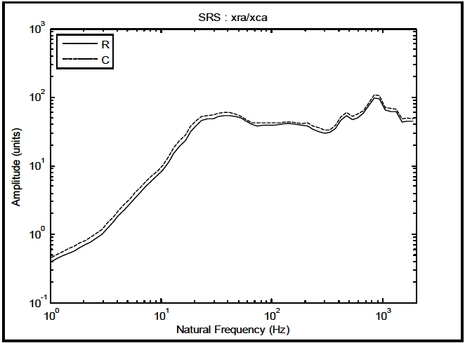
Figure description:
SRS : xra/xca
SRS : xra/xca
Legend
- R — color: black; symbol: Solid line
- C — color: black; symbol: Dashed line
| Natural Frequency (Hz) | R (Amplitude units) | C (Amplitude units) |
|---|---|---|
| 1.0 | 0.40 | 0.50 |
| 2.0 | 0.75 | 0.90 |
| 3.0 | 1.10 | 1.40 |
| 5.0 | 2.50 | 3.20 |
| 7.0 | 4.50 | 5.80 |
| 10.0 | 10.00 | 13.00 |
| 15.0 | 25.00 | 32.00 |
| 20.0 | 45.00 | 52.00 |
| 30.0 | 52.00 | 58.00 |
| 40.0 | 55.00 | 62.00 |
| 60.0 | 45.00 | 50.00 |
| 80.0 | 40.00 | 44.00 |
| 100.0 | 41.00 | 45.00 |
| 150.0 | 43.00 | 46.00 |
| 200.0 | 41.00 | 44.00 |
| 300.0 | 30.00 | 35.00 |
| 400.0 | 45.00 | 52.00 |
| 450.0 | 58.00 | 65.00 |
| 550.0 | 50.00 | 58.00 |
| 700.0 | 65.00 | 75.00 |
| 850.0 | 100.00 | 115.00 |
| 1000.0 | 70.00 | 82.00 |
| 1300.0 | 65.00 | 72.00 |
| 1500.0 | 45.00 | 52.00 |
| 2000.0 | 46.00 | 53.00 |
Notes: The chart is a log-log plot representing a Shock Response Spectrum (SRS. The X-axis represents Natural Frequency in Hertz (Hz on a logarithmic scale from 1 to 2000. The Y-axis represents Amplitude in units on a logarithmic scale from 0.1 to 1000. There are two data series, 'R' and 'C', where 'C' consistently maintains a slightly higher amplitude than 'R' across the spectrum.))
|
Figure 525.2A-23b. Composite maximax acceleration SRS for r and c.
MIL-STD-810H METHOD
525.2 ANNEX A
Since ESD estimates provide a way of comparing shock type events, Figure 525.2A-24 provides a composite of r and c ESD estimates, while Figure 525.2A-25 provides the ESD estimate for "s." It is clear from both of these plots that the most substantial error is found in the low frequency region. This is not surprising since the transfer function used to compensate the entire time trace was likely not optimal for the shock.
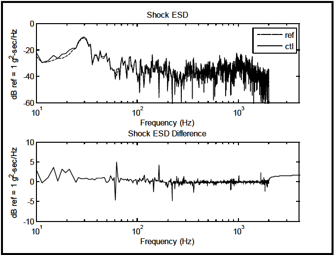
Figure description:
Shock ESD and Shock ESD Difference Analysis
Shock ESD
Legend
- ref — color: black; symbol: Dashed line
- ctl — color: black; symbol: Solid line
| Frequency (Hz) | ref (dB ref = 1 g²-sec/Hz) | ctl (dB ref = 1 g²-sec/Hz) |
|---|---|---|
| 10 | -22 | -22 |
| 12 | -29 | -27 |
| 15 | -28 | -24 |
| 18 | -27 | -25 |
| 20 | -26 | -24 |
| 22 | -24 | -22 |
| 25 | -22 | -18 |
| 28 | -15 | -16 |
| 30 | -10 | -11 |
| 35 | -15 | -16 |
| 40 | -25 | -24 |
| 45 | -28 | -23 |
| 50 | -25 | -22 |
| 55 | -28 | -25 |
| 60 | -40 | -38 |
| 65 | -35 | -36 |
| 70 | -34 | -35 |
| 80 | -30 | -32 |
| 100 | -28 | -27 |
| 150 | -35 | -33 |
| 200 | -38 | -37 |
| 300 | -40 | -42 |
| 400 | -36 | -35 |
| 500 | -35 | -34 |
| 700 | -32 | -33 |
| 1000 | -32 | -31 |
| 1500 | -40 | -41 |
| 2000 | -40 | -39 |
Shock ESD Difference
| Frequency (Hz) | Shock ESD Difference (dB ref = 1 g²-sec/Hz) |
|---|---|
| 10 | 3 |
| 12 | 0 |
| 15 | 4 |
| 18 | 0 |
| 20 | 3 |
| 22 | 2 |
| 25 | 3 |
| 28 | 0 |
| 30 | 1 |
| 40 | 1 |
| 50 | 1 |
| 60 | -5 |
| 65 | 5 |
| 70 | 0 |
| 80 | 1 |
| 100 | 1 |
| 150 | -2 |
| 180 | 4 |
| 200 | 0 |
| 250 | -5 |
| 300 | 1 |
| 400 | 1 |
| 500 | 0 |
| 700 | 0 |
| 800 | -2 |
| 1000 | 1 |
| 1500 | 0 |
| 1800 | -2 |
| 2000 | 1.5 |
| 3000 | 1.8 |
Notes: The plots represent energy spectral density (ESD of a shock event and the difference between a reference signal and a control signal across a frequency spectrum on a logarithmic scale.)
|
Figure 525.2A-24. ESD estimates for r and c.
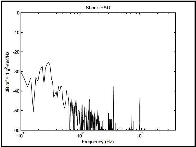
Figure description:
Shock ESD
Shock ESD
| Frequency (Hz) | Shock ESD (dB ref = 1 g²-sec/Hz) |
|---|---|
| 10.0 | -30.0 |
| 12.0 | -35.2 |
| 14.1 | -37.9 |
| 15.0 | -33.3 |
| 16.5 | -42.4 |
| 17.5 | -50.8 |
| 19.5 | -33.1 |
| 21.6 | -34.8 |
| 24.3 | -28.5 |
| 26.5 | -27.3 |
| 29.5 | -25.2 |
| 33.5 | -33.9 |
| 37.8 | -43.1 |
| 43.5 | -40.1 |
| 47.9 | -37.2 |
| 52.5 | -42.8 |
| 57.5 | -48.8 |
| 64.6 | -39.9 |
| 72.4 | -55.2 |
| 81.3 | -44.2 |
| 91.2 | -52.7 |
| 100.0 | -55.8 |
| 120.2 | -53.3 |
| 141.3 | -44.2 |
| 165.9 | -51.2 |
| 186.2 | -54.3 |
| 208.9 | -49.8 |
| 251.2 | -57.8 |
| 302.0 | -51.3 |
| 354.8 | -37.6 |
| 421.7 | -60.0 |
| 501.2 | -60.0 |
| 631.0 | -60.0 |
| 741.3 | -52.6 |
| 851.1 | -55.3 |
| 1000.0 | -43.3 |
| 1122.0 | -60.0 |
Notes: The chart shows a spectral density plot with a logarithmic x-axis (Frequency in Hz and a linear y-axis (dB ref = 1 g²-sec/Hz. The plot contains numerous peaks and troughs, with prominent spikes occurring around 350 Hz and 1000 Hz.))
|
Figure 525.2A-25. ESD estimate for s.
MIL-STD-810H METHOD
525.2 ANNEX A
525.2 ANNEX B METHOD 525.2, ANNEX B SUMMARY OF POST-TEST ANALYSIS PROCESSING PROCEDURES AND TEST TOLERANCE SPECIFICATION
525.2 ANNEX B
place, however for averaging windows on the order of the oversample factor bias error should be minimal. Whenever practical bias errors in the estimates for the error assessment need to be minimized. If there exists questions relative to the size of normalized bias and random errors, much more detailed processing beyond the scope of this Annex may need to be employed (paragraph 6.1, reference a).
In description of the error assessment expressions, the designation “local” or “global” is made. The term “local” refers to a statistic that is useful for processing short segments of time-varying traces, while the term “global” refers to a statistic that is better suited to summarizing overall time traces. For example, the collection of STA for root-mean-square provides “local” estimates related to a potential tolerance specification. The cumulative probability density function estimate for describes error as being perhaps Gaussian or non-Gaussian. This is a “global” assessment from which a tolerance specification might be based upon the distributional form of the estimate. Generic variables
, and
are employed in the formulas whereby , and may be substituted at will depending upon interpretation. In the formulas to follow will be an "index" related to the time sample interval for the time average estimate (it is a time shift parameter for averaging) and will be the number of time points averaged over. is the greatest integer designation for . It is assumed that where generally M is an odd number to prevent any phase shift introduced in the processing.
There are three cases in which joint consideration of deterministic and stochastic may be useful. In the first case a scatterplot constructed by plotting the point in the plane will reveal valuable information relative to a single plot of the error . In the second case since computation of an ASD/ESD estimate over a deterministic time trace has some meaning the comparison of the ASD/ESD estimates for and may provide meaningful information in relation to the ASD/ESD for . In particular the deterministic estimate is divided into the stochastic estimate to examine the ratio in the frequency domain. Finally, comparison of SRS estimates for versus along with an SRS estimate for i.e., the "noise" can be useful.
For easy reference the following table is provided:
Table B-I. Summary of error assessment expressions
| E1 | MEAN (local & global) S |
| E2 | ROOT-MEAN-SQUARE & MEAN-SQUARE (local & global) S |
| E3 | COVARIANCE, CORRELATION and SCATTER-PLOT (global) R and C |
| E4 | PROBABILITY DENSITY, CUMULATIVE PROBABILITY and QUANTILE (global) S |
| E5 | FRACTION-OF-TIME (global) S |
| E6 | ASD/ESD/PERIODOGRAM (global) R and C |
| E7 | SHOCK RESPONSE SPECTRA (global) R and C |
Expressions E1 through E7 are potentially useful for TWR tolerance specification. Future editions of MIL-STD-810 will likely refine and add to these expressions as SESA TWR testing becomes more common and experience with both replication error assessment and subsequent test specification becomes more common. Generally E1, E2 E5, E6, and E7 will directly relate to tolerance specification. E3 and E4 provide good qualitative information but will not directly relate to tolerance specification.
MIL-STD-810H METHOD
525.2 ANNEX B
E1: MEAN (local & global)
A collection of STA for provides an indication of any potential “shift” in very low frequency information contained in under TWR. A zero mean error is desirable otherwise bias may be present. The mean estimate for is defined as follows: \hat{\mu}_{x}(t_{i})=\int\limits_{T_{i-1}}^{T_{i}}x(t)dt\left.rightarrow\hat{m}_{x_{i}}=\frac{1}{N_{a}}\sum\limits_{i=M-[N_{a}/2]+1}^{M+[N_{a}/2]}x(t_{i}) (1) The normalized random error in the mean estimate in units of root-mean-square is defined as for , overall bandwidth of , and , averaging time. (2) Note that this is related to the confidence interval with confidence coefficient on the mean of a population (not necessarily a time history) obtained by a sample of size i.e.,
E2: ROOT-MEAN-SQUARE and MEAN-SQUARE (local & global)
A collection of STA root-mean-square levels in time is fundamental for replication error assessment and probably is closely aligned with vendor TWR error assessment. It is basically a “rms” error. The mean-square error assessment is included for completeness but is generally not particularly useful.
The root-mean-square of with zero mean over a short interval of time is computed as follows:
\right.
and the normalized random error for the root-mean-square estimate is given by,
for , overall bandwidth of , and , averaging time.
This estimate is essentially an estimate of the standard deviation of the time trace over a short time interval.
The mean-square of with zero mean over a short interval of time is computed as follows:
For overall bandwidth B in Hz and averaging time I in seconds, the normalized random error for the mean-square estimate is given by
1 ε[Ÿ²]~- (5) BT
This estimate is essentially an estimate of the variance of the time trace over a short time interval. That is the confidence interval with confidence coefficient 1-α on the standard deviation of a population (not necessarily a time history) obtained by a sample of size N, i.e.,
MIL-STD-810H METHOD
525.2 ANNEX B
for .
For application for and or 0.1 seconds the normalized random error for a mean comparable to the standard deviation, root-mean-square and mean-square is respectively for averaging time of 0.01 seconds, and respectively for averaging time of 0.1 seconds. To obtain a meaningful characterization of , it is important the normalized random error be minimized by as long an averaging time as is consistent with nominal bias error.
E3: COVARIANCE, CORRELATION, and SCATTER-PLOT (global and local)
Generally, covariance and correlation can be viewed as meaningful in the case of regression between a deterministic and a random time trace i.e., and Since no new information is added by computing the correlation or covariance between and . Covariance and correlation should be viewed in terms of a "regression fit" of to . This particular replication error assessment is somewhat qualitative thus not particularly useful for tolerance specification e.g., specifying a correlation coefficient for tolerance would be too gross a parameter to be meaningful. The covariance relationship between two time traces over a short interval of time (local covariance), or over the entire time trace (global covariance) is computed in the time domain as follows:
This quantity can be normalized to provide the local or global correlation coefficient that can be expressed as follows:
The time trace basis for these expressions from traditional data analysis is as follows. For two arbitrary random processes and whose sample functions are indexed on and for which the ensemble means are defined by and where expectation is over index then the cross covariance function at arbitrary fixed values of and is given by
If _ 7 = 0 then C¸„ (t,t) = E[(x (1)− µx (1))(yk (1) — µ, (1))] = C (1), and this is of the form of the covariance xy μx expression above only where the expected value is not over an ensemble indexed on k, but over a finite time interval of length Nat. The expression for xy is merely a “normalized” version of the expression for cov(x,y) defined above. When the kth sample functions x (i^t) and y/ (i^t) for i = 1, 2,..., N are plotted on the x and y axes, respectively, the resulting plot is termed a "scatter-plot." The "scatter-plot" depicts the degree of covariance or correlation between two time traces. For xy in the neighborhood of zero there tends to be no correlation between time traces, and the "scatter-plot" reveals an ellipse with major and minor axes approximately equal. For a distribution of rxy close to either -1 or +1, there is substantial correlation between the time traces, and the "scatter-plot" provides an ellipse with a very small minor axis. In general "scatter-plot" information at the amplitude extremes is of most interest since this defines the correspondence between time trace peaks and valleys.
MIL-STD-810H
METHOD 525.2 ANNEX B
E4: PROBABILITY DENSITY, CUMULATIVE PROBABILITY, and QUANTILE (global)
A probability density function estimate is generally termed a histogram. A useful indicator of the form of time trace amplitudes is the histogram and its counterpart, the cumulative histogram. Generally, this analysis display is useful only for stationary time traces of substantial duration, e.g., 5 seconds or more. Time traces with even small time-varying root-mean-square levels almost always invalidate this procedure unless some finite distribution mixture can be specified. The histogram is useful usually when it is compared to a theoretical probability density function of an assumed form, e.g., the Normal probability density function. With time trace amplitude bins along the horizontal axis, and “bin counts” along the vertical axis, the logarithm of the bin counts may be used to examine the (1) shape of the histogram for the mid bin ranges, and (2) difference in tails for the small amplitude and the large amplitude bins. Because the probability structure of the difference can be so important in assessing the nature of TWR error, a rather complete discussion of its statistics is provided here. The probability density and probability estimate of are defined as follows:
From paragraph 6.1, reference a, the probability of taking values between and during time interval (where " " is amplitude level and " " is a width designation for a time trace amplitude) is estimated as:
with . The probability density is defined as:
From this development, the cumulative probability density and probability density are related as follows:
N
θ [a] = Ĵ î¸ (5)d5 ↔ ¸[a] = Σî¸[a]pa (11)
-00 i=1
The normalized mean square random error for the probability density estimate is given from paragraph 6.1, reference a as follows:
c² 2BTWp (a) where, for continuous bandwidth with noise c≈0.3. Since probability density estimates are particularly susceptible to bias error, the mean square bias error is given as
W p(a) 576 px (a) for P. (a) the second derivative of evaluated På at “a”. (12)
It may be useful to compare the probability structure of ( )
x t directly to a known probability structure such as the Normal probability density/distribution. This can be done in this formulation by merely plotting the estimated probability structure of ( ) x t along with the selected theoretical probability structure. There are both parametric and nonparametric statistical tests that allow comparison of probability structures at selected levels of significance. In particular, the nonparametric Kolmogorov-Smirnov test provides a basis for comparison of two sample probability distribution estimates or one sample probability distribution estimate with a theoretical probability distribution estimate. It is possible to use statistical hypothesis testing for purposes of tolerance specification provided the properties of such statistical tests are well understood and such tolerance specification is meaningful.
A strong visual test for equivalence of reference and control distributions is a plot of the quantiles of the two time history trace cumulative distribution probability functions, and is termed a quantile-quantile (q-q) plot. The quantile is defined in terms of the probability distribution function as follows:
MIL-STD-810H
METHOD 525.2 ANNEX B
For the probability distribution function with probability density function , the quantile of is defined as follows:
and similarly, for the probability distribution with probability density function , the quantile of is defined as:
For a given quantile , the plot of versus on a rectangular axis is termed a " plot." and may be both analytical, both empirical (estimated from data), or a combination of analytical and empirical.
Examination of the “tails” or extreme values (peaks and valleys) along with the fit to a theoretical Gaussian distribution function, provides the most useful information.
Application of this procedure is most common for plotting the quantiles of the distribution of s(t) against those of the Gaussian distribution function. It is also useful for empirical estimates of r(t) and c(t) against one another, or r(t) and c(t) separately against the Gaussian distribution quantiles. It is important to remember that in all such plots, particularly between r(t) and c(t) time correlation information is lost. It is noted that once the "probability" function of s(t) is established then higher order moments related to skewness or kurtosis can be established.
E5: FRACTION-OF-TIME (global)
Closely related to the probability/quantile amplitude assessment in E4 is the Fraction-of-Time (FOT) assessment. For the FOT estimate of the error is above a certain magnitude and is assessed more intuitively and directly. It is also important to note that for FOT assessment, generally no theoretical distributional form is attached to the FOT estimate e.g., FOT is never spoken of as being Gaussian distributed, etc. For statistical analysis of time series the FOT assessment replaces the more traditional probability analysis., however, FOT distribution is a valid probability distribution function. For processing on a statistical basis the Fraction-of-Time (FOT) is defined as follows:
measure{u =[t,t+T]: x(u)≤ §} _ 1 µ:+T, F₁ (t; 5; x) = = ±±ƒ‚³ U (≤ − x (u))du (15) measure ire{u = [t,t+T]}
where
T≥O U (t) = elsewhere
For the error time trace, s(t), FOT allows assessment of the percentage of time the error is above a certain level and a
correct display would indicate the times along the reference time trace r(t) for which this occurs. Generally, this is summarized in a single plot similar to the probability based cumulative distribution function estimate. Thus if
Fr(ts)≤ 0.05 and Fr (t; §2;s) ≥ 0.05 then s(t) lies between 5, and ½₂ ninety percent of the TWR test time where it is assumed ₁ and can be related to some level of the reference e.g., the range of the reference, for purposes of developing a test specification on replication error.
MIL-STD-810H METHOD
525.2 ANNEX B E6: ASD/ESD/PERIODOGRAM (global)
For a deterministic time trace such as a frequency domain estimate is meaningful and similar to the fitting of a Fourier series to an analytically defined function. Visual comparison between frequency domain estimates for and can be made and the ratio of the estimates at each frequency line provided by ratioing the computed quantities (this must never be interpreted as a “transfer function estimate” between the reference and the control time traces).It might be noted that for TWR the “transfer function estimate” is provided in the vendor software in the form of the frequency domain Fourier “drive signal compensation” function. The frequency domain estimates provide for tolerance specification that is directly related to tolerance specifications in Method 514. The basic definition of the windowed two-sided periodogram for an point digital sequence in continuous frequency form is as follows:
Generally the two-sided periodogram is made one sided by multiplying by a factor of 2 with 0≤ f≤0.5, and the periodogram is sampled at discrete frequencies, f, for i = 0,1,2,..., N/2 with a uniform spacing of Af = 1/NAt. The ASD and ESD can be defined in terms of the sampled periodogram. An ASD estimate is typically a time average sampled periodogram estimate over a limited time interval, with an applied window to reduce spectrum leakage. For stationary time traces the ASD represents a powerful means of comparison between r(t) and c(t), and a display of the frequency content in s(t). Paragraph 6.1, reference a provides information on ASD processing of stationary time traces including normalized random and bias error estimates. For analysis filter bandwidth B in Hz, and averaging time T in seconds, the normalized random error for the ASD estimate is given by
(17)
while the normalized bias error is given by
(18)
where
is an estimate of the half-power bandwidth of a resonant peak.
An ESD estimate is typically a scaled periodogram, scaled by multiplying the periodogram by the duration of the time trace , over a very short transient time trace that cannot be characterized by an ASD estimate. A uniform or end tapered uniform time window is generally placed over the significant portion of the time trace. For transient TWR time traces, ESD estimates are useful for comparing and in addition to examining the character of .
E7: SRS – Shock Response Spectra (global)
As in the case of the frequency domain estimates in E6 a comparison between SRS estimates for deterministic r(t) and stochastic c(t) can be made. The SRS estimate for the error time trace s(t) is related to an SRS estimate for pre-shock and post-shock considered to be random in nature (see Method 516).The SRS may be expressed as a time domain convolution of an impulse response function that has the character of the response to base-input of the mass of a single- degree-of-freedom mechanical system, with a certain percentage of critical damping. The SRS estimate is a function of the output of the mass displacement, velocity, and acceleration. If the maximum absolute acceleration (positive or negative) is selected over the time interval of excitation, and plotted versus the undamped natural frequency of the single-degree-of-freedom system, the resulting plot over a selected set of frequencies is referred to as a maximax
MIL-STD-810H METHOD
525.2 ANNEX B
shock response spectrum. It is becoming increasingly evident that for most cases of mechanical shock the pseudo- velocity SRS estimate is a more indicative measure of potential for mechanical damage (because mechanical damage is related to mechanical stress that, in turn, is proportional to relative velocity of a mass-spring-damper system). Various references provide the details of SRS computation. For transient time trace TWR comparison, the SRS of r(t) and c(t) is useful and demonstrates the faithfulness of shock reproduction under TWR. Computing the SRS for s(t) is less useful and difficult to interpret since random variable S should represent a noise source but not Normal distributed. The mathematics for the SRS computation over a transient ( ) for 0 x t ≤≤ t T r is given as follows:
SRS (ƒ„,5) = I[y(t, ƒ„‚5)]=: I (t-t)x(t)dr | for 0≤T, ≤T for
where,
SRS (f.) the magnitude of the SRS at natural frequency fr
I a nonlinear functional operating on the resulting convolution y(t,ƒ„‚5)
h(t) impulse function response for a damped single-degree-of-freedom system with base input and undamped natural frequency for having damping ratio 5.
x(7) finite input record 0≤t≤T
T time of response assessment where generally T, <T
Natural frequency, nf , can extend beyond the sampling frequency of x(t). The SRS estimate is computed through filtering a transient time record, and does not have a clear random error or bias error criterion. Numerically, the time trace sample rate should be ten times the bandwidth of the time trace in order to provide an acceptable error in the estimates (approximately 5 percent error).