525.2-6 TPP TRANSIENT VIBRATION
Figure 525.2A-10 displays the transient vibration time trace information, from which the general form of the transient vibration is preserved, and the difference is reasonably nominal. There is an apparent low frequency component in the time traces between 5.58 and 5.70 seconds. Such a dominant low frequency component could preclude strict product model assumptions for post processing. However, generally, the product model is reasonably robust with regard to change of frequency, i.e., the momentary change in frequency character is averaged in over the entire record length.
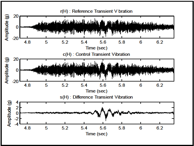
Figure description:
r(H : Reference Transient V bration
| Time (sec) | Amplitude (g) |
|---|---|
| 4.72 | 0.0 |
| 4.80 | 0.2 |
| 4.90 | 4.5 |
| 5.00 | 9.0 |
| 5.10 | 11.5 |
| 5.20 | 14.0 |
| 5.30 | 11.0 |
| 5.40 | 13.0 |
| 5.50 | 8.5 |
| 5.55 | -5.5 |
| 5.60 | 15.8 |
| 5.63 | -18.2 |
| 5.68 | 13.5 |
| 5.72 | -2.8 |
| 5.80 | 10.0 |
| 5.90 | 7.2 |
| 6.00 | 8.8 |
| 6.10 | 5.2 |
| 6.20 | 4.5 |
| 6.30 | 2.8 |
| 6.35 | 2.2 |
c(H : Control Transient Vibration
| Time (sec) | Amplitude (g) |
|---|---|
| 4.72 | 0.0 |
| 4.80 | 0.1 |
| 4.90 | 4.4 |
| 5.00 | 8.9 |
| 5.10 | 11.4 |
| 5.20 | 13.9 |
| 5.30 | 10.9 |
| 5.40 | 12.8 |
| 5.50 | 7.7 |
| 5.55 | -4.0 |
| 5.60 | 13.7 |
| 5.63 | -15.3 |
| 5.68 | 11.7 |
| 5.72 | -2.3 |
| 5.80 | 9.8 |
| 5.90 | 7.1 |
| 6.00 | 8.7 |
| 6.10 | 5.1 |
| 6.20 | 4.4 |
| 6.30 | 2.7 |
| 6.35 | 2.1 |
s(H : Difference Transient Vibration
| Time (sec) | Amplitude (g) |
|---|---|
| 4.72 | 0.0 |
| 4.80 | 0.1 |
| 4.90 | 0.1 |
| 5.00 | 0.1 |
| 5.10 | 0.1 |
| 5.20 | 0.1 |
| 5.30 | 0.1 |
| 5.40 | 0.2 |
| 5.50 | 0.8 |
| 5.55 | -1.5 |
| 5.60 | 2.1 |
| 5.63 | -2.9 |
| 5.68 | 1.8 |
| 5.72 | -0.5 |
| 5.80 | 0.2 |
| 5.90 | 0.1 |
| 6.00 | 0.1 |
| 6.10 | 0.1 |
| 6.20 | 0.1 |
| 6.30 | 0.1 |
| 6.35 | 0.1 |
Figure 525.2A-10. Transient vibration time traces - r, c, and s.
The rudimentary overall maximum and minimum statistics for the transient vibration time trace are as follows: r min/max -17.50/15.41; c(H) min/max -18.12/16.11; and s(H) min/max -2.99/2.12.
The replication error is assessed under the product model assumption as follows:
- a. Plot for r versus c (cross-plot) is generated to measure strength of TPP correlation (particularly for peaks and valleys at extremes of the cross-plot).
- b. qq-plot for s is generated to examine the difference time trace for normality.
- c. Root-mean-square envelopes are generated at 0.1 second averaging time for r and c under a product model assumption.
- d. Normalized ASD estimates are determined for r and c under a product model assumption.
Figure 525.2A-11 plots the amplitude of r versus the amplitude c. Each individual point in the plot represents a point in time with r amplitude along the horizontal axis, and c amplitude along the vertical axis. The spread along the minor axis of this ellipsoidal form implies the difference in r and c at several time increments. In this particular case, the negative peak spread near -18g is nominal, whereas the positive peak spread near 14g demonstrates up to a 2g difference at given time increments. The spread near rc≈0 is of little concern since the signal-to-noise ratio is small, and statistically independent Gaussian noise samples are being scatter plotted.
MIL-STD-810H METHOD 525.2 ANNEX A
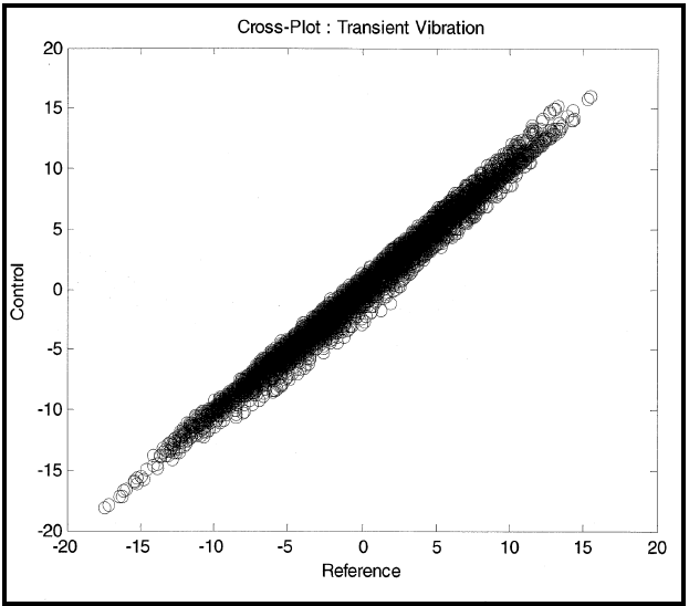
Figure description:
Cross-Plot : Transient Vibration
Cross-Plot : Transient Vibration
| Reference | Control |
|---|---|
| -17.8 | -18.1 |
| -16.5 | -17.2 |
| -15.4 | -16.0 |
| -14.2 | -14.5 |
| -13.1 | -13.8 |
| -11.8 | -12.5 |
| -10.5 | -10.9 |
| -9.2 | -9.8 |
| -8.0 | -8.5 |
| -6.7 | -7.2 |
| -5.4 | -5.8 |
| -4.1 | -4.5 |
| -2.8 | -3.2 |
| -1.5 | -1.9 |
| -0.2 | -0.5 |
| 1.1 | 0.8 |
| 2.4 | 2.1 |
| 3.7 | 3.5 |
| 5.0 | 4.8 |
| 6.3 | 6.2 |
| 7.6 | 7.5 |
| 8.9 | 8.9 |
| 10.2 | 10.2 |
| 11.5 | 11.6 |
| 12.8 | 13.0 |
| 14.1 | 14.3 |
| 15.4 | 15.7 |
| 15.8 | 16.1 |
Notes: The chart is a dense scatter plot showing a strong positive linear correlation between the 'Reference' and 'Control' variables. Data points are clustered tightly around the y = x line across the range from approximately -18 to +16 on both axes.
Figure 525.2A-11. r versus c cross-plot.
Figure 525.2A-12 displays the quantiles of s versus the Gaussian distribution. This figure clearly reveals that the difference between r and c is non-Gaussian, and this complicates the replication error assessment. In particular, “s” has tails that are longer that those that might be expected for a Gaussian distribution with a mean and standard deviation estimated from s.
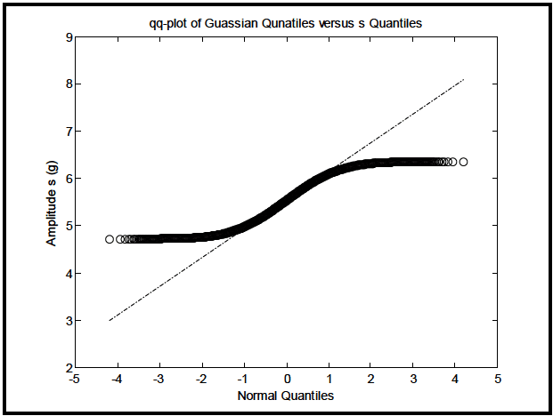
Figure description:
qq-plot of Guassian Qunatiles versus s Quantiles
qq-plot of Guassian Qunatiles versus s Quantiles
Annotations
- Reference line for normal distribution (reference_line - position: y = 0.6x + 5.5)
| Normal Quantiles | Amplitude s (g) | Reference Line |
|---|---|---|
| -4.2 | 4.71 | 2.98 |
| -4.0 | 4.71 | 3.10 |
| -3.5 | 4.72 | 3.40 |
| -3.0 | 4.73 | 3.70 |
| -2.5 | 4.75 | 4.00 |
| -2.0 | 4.81 | 4.30 |
| -1.5 | 4.93 | 4.60 |
| -1.0 | 5.08 | 4.90 |
| -0.5 | 5.28 | 5.20 |
| 0.0 | 5.50 | 5.50 |
| 0.5 | 5.72 | 5.80 |
| 1.0 | 5.92 | 6.10 |
| 1.5 | 6.07 | 6.40 |
| 2.0 | 6.19 | 6.70 |
| 2.5 | 6.25 | 7.00 |
| 3.0 | 6.27 | 7.30 |
| 3.5 | 6.28 | 7.60 |
| 4.0 | 6.29 | 7.90 |
| 4.2 | 6.30 | 8.02 |
Notes: The chart displays a quantile-quantile (Q-Q plot. The 'Amplitude s' data points follow an S-curve, deviating from the linear reference line at the tails, which indicates that the distribution of 's' has shorter tails (is more bounded than a normal distribution. Note the spelling errors in the original chart title ('Guassian' and 'Qunatiles'.)))
|
Figure 525.2A-12. Transient vibration q-q plot for s versus Gaussian.
MIL-STD-810H METHOD
6.1 Referenced Documents
- a. Bendat, Julius S. and Allan G. Piersol, Random Data Analysis and Measurement Procedures, 4th Edition, John Wiley & Sons, Inc., New York, 2010.
- b. Handbook for Dynamic Data Acquisition and Analysis, IEST-RD-DTE 012.2, Institute of Environmental Sciences and Technology, Arlington Place One, 2340 S. Arlington Heights Road, Suite 100, Arlington Heights, IL 60005-4516.
- c. Merritt, Ronald G., "Application of Mixed Effects Models to a Collection of Time Trace Product Models," Proceedings of the 77th Shock and Vibration Symposium, Nov. 2006; Shock & Vibration Exchange (SAVE), 1104 Arvon Road, Arvonia, VA 23004.
- d. Stuart, Alan and J. Keith Ord, Kendall’s Advanced Theory of Statistics, 5th Edition Volume 1 Distribution Theory, Oxford University Press, New York NY, 1987.
6.2 Related Documents
- a. Bickle, Larry W. and Ned R. Keltner, Estimation of Transient Measurement Errors, SAND78-0497, August 1978.
- b. Shock and Vibration Handbook, 5th Edition, Edited by Cyril M. Harris and Allan G. Piersol, McGraw-Hill, New York NY, 2002.
- c. Egbert, Herbert W. "The History and Rationale of MIL-STD-810 (Edition 2)", January 2010; Institute of Environmental Sciences and Technology, Arlington Place One, 2340 S. Arlington Heights Road, Suite 100, Arlington Heights, IL 60005-4516.
(Copies of Department of Defense Specifications, Standards, and Handbooks, and International Standardization Agreements are available online at https://assist.dla.mil.
Requests for other defense-related technical publications may be directed to the Defense Technical Information Center (DTIC), ATTN: DTIC-BR, Suite 0944, 8725 John J. Kingman Road, Fort Belvoir VA 22060-6218, 1-800-225-3842 (Assistance--selection 3, option 2), http://www.dtic.mil/dtic/; and the National Technical Information Service (NTIS), Springfield VA 22161, 1-800-553-NTIS (6847), http://www.ntis.gov/.
Downloaded from https://www.everyspec.com
MIL-STD-810H METHOD 525.2
(This page is intentionally blank.)
MIL-STD-810H
METHOD 525.2 ANNEX A METHOD 525.2, ANNEX A SESA POST-TEST ANALYSIS ILLUSTRATION FOR TEST TOLERANCE ASSESSMENT