9.9.1
FATIGUE — Separate data presentations are made for strain-controlled and load-controlled data. The only case where load-controlled data can be presented with strain-controlled data is when long-life tests have been switched from strain to load control in accordance with recommended procedures (see Section 9.2.5.1). Separate plots should be constructed for each material, notch concentration (in the case of load-controlled data), temperature, or other documented parameters that have been demonstrated to cause significant variations in fatigue behavior.
Load-controlled data presentations should consist of a family of at least three stress ratio or mean stress curves, with at least six data points per curve covering two orders of magnitude in life. (See exceptions noted in Section 9.2.3.5.1). The basic data should be included on each plot, with separate symbols used for each stress ratio or mean stress. Runouts should be identified with an arrow (→). The analytically defined mean S/N curves for each stress ratio or mean stress should also be included on each plot. These curves should not be extrapolated beyond existing data.
The fatigue curve for each stress ratio should be constructed based on the following criteria:
- (1) The curve should start at the greatest maximum stress for that specific stress ratio. Unnotched fatigue curves should not extend above the average tensile ultimate strength of the material.
- (2) The curve will terminate at the lowest maximum stress or longest life value, whichever is most limiting for that specific stress ratio.
In addition to the stress-life plot [such as shown in Figure 9.9.1.1(e)], a tabulation of test and material conditions should also be included. At a minimum the following information should be included with an S/N plot:
- (1) Material
- (2) Product Form, Grain Direction, Thickness, Processing History, Fabrication Sequence
- (3) Test Parameters
- Loading
- Test Frequency
- Temperature
- Environment
- (4) Average Tensile Properties
- (5) Specimen Details
- Notch Description
- Specimen Dimensions
- (6) Surface Condition/Surface Residual Stresses/Finish
- Finish
- Residual Stress Data
- (7) Equivalent Stress Equation
- Life Equation With Parameter Estimates
- Standard Deviation of log(Life)
- Adjusted R-Squared Statistic
- Sample Size
- (8) Reference Numbers
- (9) No. of Heats/Lots
The following cautionary note should be included with each equivalent stress equation: [Caution: The equivalent stress model may provide unrealistic life predictions for maximum stresses and stress ratios
MIL-HDBK-5J
9.9.1.1
Load Control — A large collection of 300M alloy die forging fatigue data is presented in Figure 9.9.1.1(a). The required steps for the analysis of the data set are presented below.
MIL-HDBK-5J
9.9.1.2
Strain Control —A collection of iron alloy bar strain-controlled fatigue data at 70 °F is given in Table 9.9.1.2. The required steps for the analysis of the data set are presented below. The guideline sections relating to each step in the analysis are noted.
Data Requirements (See Section 9.2.4.8) — The data set includes three strain ratios (Rₑ = -1.0, 0.0, 0.6) each consisting of at least eight nonrunout data points. This satisfies the minimum recommended sample size for analysis. Two runouts (Nf = 10⁵ and 10⁶ at Rₑ = -1 are included in the data set.
Data Collection (See Section 9.6.1.1)—The specimen design for the test program is reported as uniform-gage section with a diameter of 0.20 inches. Failure is defined as complete separation. The tensile properties are presented in the correlative information. No information is available regarding the fabrication sequence for the specimens. Fabrication information is important, although in this case it is not considered sufficient cause to reject the data set for analysis. The test data at the strain ratio provide information regarding this material's cyclic stress-strain response. The cyclic stress-strain curve constructed from the data is shown in Figure 9.9.1.2(a). The monotonic curve (dashed) is estimated from the reported yield and ultimate strengths.
MIL-HDBK-5J
31 January 2003
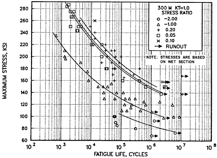
Figure description:
Fatigue Life of 300 M Steel
300 M KT=1.0
Legend
- STRESS RATIO -2.00 — color: black; symbol: Open Circle
- STRESS RATIO -1.00 — color: black; symbol: Open Triangle
- STRESS RATIO 0.20 — color: black; symbol: Plus (+
- STRESS RATIO 0.05 — color: black; symbol: Open Square
- STRESS RATIO 0.10 — color: black; symbol: Cross (x
- RUNOUT — color: black; symbol: Right Arrow
Annotations
- NOTE: STRESSES ARE BASED ON NET SECTION (text_label - position: right middle)
- 300 M KT=1.0 (text_label - position: top right)
| Stress Ratio | Fatigue Life (Cycles) | Maximum Stress (KSI) | Runout |
|---|---|---|---|
| -2.00 | 65000 | 100 | No |
| -2.00 | 75000 | 90 | No |
| -2.00 | 85000 | 85 | No |
| -2.00 | 300000 | 80 | No |
| -2.00 | 7000000 | 73 | No |
| -2.00 | 1200000 | 93 | Yes |
| -2.00 | 1200000 | 68 | Yes |
| -1.00 | 1200 | 235 | No |
| -1.00 | 1400 | 210 | No |
| -1.00 | 1500 | 200 | No |
| -1.00 | 1600 | 196 | No |
| -1.00 | 4000 | 190 | No |
| -1.00 | 8000 | 175 | No |
| -1.00 | 9000 | 160 | No |
| -1.00 | 17000 | 150 | No |
| -1.00 | 25000 | 150 | No |
| -1.00 | 25000 | 140 | No |
| -1.00 | 30000 | 130 | No |
| -1.00 | 35000 | 150 | No |
| -1.00 | 45000 | 155 | No |
| -1.00 | 60000 | 140 | No |
| -1.00 | 60000 | 130 | No |
| -1.00 | 75000 | 140 | No |
| -1.00 | 100000 | 110 | No |
| -1.00 | 110000 | 140 | No |
| -1.00 | 130000 | 120 | No |
| -1.00 | 150000 | 130 | No |
| -1.00 | 170000 | 110 | No |
| -1.00 | 200000 | 130 | No |
| -1.00 | 220000 | 115 | No |
| -1.00 | 250000 | 120 | No |
| -1.00 | 400000 | 110 | No |
| -1.00 | 550000 | 125 | No |
| -1.00 | 650000 | 120 | No |
| -1.00 | 1300000 | 110 | No |
| -1.00 | 2000000 | 125 | No |
| -1.00 | 2700000 | 98 | No |
| -1.00 | 4000000 | 120 | No |
| -1.00 | 5500000 | 100 | No |
| -1.00 | 8000000 | 100 | No |
| -1.00 | 1200000 | 107 | Yes |
| -1.00 | 4500000 | 98 | Yes |
| -1.00 | 10000000 | 100 | Yes |
| 0.20 | 10000 | 250 | No |
| 0.20 | 15000 | 240 | No |
| 0.20 | 25000 | 220 | No |
| 0.20 | 25000 | 190 | No |
| 0.20 | 35000 | 220 | No |
| 0.20 | 40000 | 220 | No |
| 0.20 | 50000 | 210 | No |
| 0.20 | 55000 | 180 | No |
| 0.20 | 60000 | 195 | No |
| 0.20 | 65000 | 180 | No |
| 0.20 | 65000 | 210 | No |
| 0.20 | 70000 | 170 | No |
| 0.20 | 80000 | 200 | No |
| 0.20 | 80000 | 180 | No |
| 0.20 | 85000 | 210 | No |
| 0.20 | 100000 | 180 | No |
| 0.20 | 130000 | 165 | No |
| 0.20 | 450000 | 180 | No |
| 0.20 | 1500000 | 158 | Yes |
| 0.20 | 2000000 | 158 | Yes |
| 0.20 | 2500000 | 158 | Yes |
| 0.20 | 11000000 | 138 | Yes |
| 0.05 | 1500 | 288 | No |
| 0.05 | 1800 | 283 | No |
| 0.05 | 2000 | 275 | No |
| 0.05 | 2200 | 267 | No |
| 0.05 | 2200 | 250 | No |
| 0.05 | 2500 | 275 | No |
| 0.05 | 3500 | 243 | No |
| 0.05 | 4000 | 250 | No |
| 0.05 | 5000 | 250 | No |
| 0.05 | 11000 | 220 | No |
| 0.05 | 25000 | 200 | No |
| 0.05 | 35000 | 180 | No |
| 0.05 | 110000 | 160 | No |
| 0.05 | 400000 | 160 | No |
| 0.05 | 750000 | 150 | No |
| 0.05 | 1400000 | 140 | No |
| 0.05 | 2800000 | 150 | Yes |
| 0.05 | 3500000 | 138 | Yes |
| 0.10 | 15000 | 260 | No |
Figure X.X.X.X(a). Best-fit S/N curves for unnotched 300M alloy forging, ksi, longitudinal and transverse directions.
Correlative Information for Figure X.X.X.X.X
| Product Forms: | Test Parameters: |
|---|---|
| Die forging, 10 x 20 inches | Loading - Axial |
| CEVM | Frequency - 1800 to 2000 cpm |
| Die forging, 6-1/2 x 20 inches | Temperature - RT |
| CEVM | Atmosphere - Air |
| RCS billet, 6 inches CEVM | No. of Heat/Lots: |
| Forged Bar, 1.25 x 8 inches | 6 |
| CEVM | |
| Properties: | Equivalent Stress Equation: |
| TUS, ksi | Log Nf = 14.8-5.38 log (Seq-63.8) |
| 274-294 | Seq = Sa + 0.48 Sm |
| TYS, ksi | Std. Error of Estimate, Log (Life) = 55.7 (1/Seq) |
| 227-247 | Standard Deviation, Log (Life) = 1.037 |
| Temp., °F | R2 = 82.0 |
| RT | |
| Specimen Details: | |
| Unnotched | Sample Size: |
| 0.200 - 0.250 inch diameter | 104 |
| Surface Condition: | [Caution: The equivalent stress model may provide unrealistic life predictions for stress ratios beyond those represented above.] |
| Heat treat and finish grind to a surface finish of RMS 63 or better with light grinding parallel to specimen length, stress relieve | |
| References: | |
| 2.3.1.4.8(a), (c), (d), (e) |
Figure 9.9.1.1(e). Example S/N curve and correlative information
MIL-HDBK-5J
9.9.2
FATIGUE CRACK GROWTH— When preparing fatigue crack growth data proposals for submittal to the MIL-HDBK-5 Coordination Group, several steps must be taken. First, various factors potentially influencing crack-propagation rates should be documented in a fatigue crack growth Data Proposal as shown in Table 9.9.2. Second, data for individual test conditions should be plotted and compared so that a determination can be made as to whether combinations of test conditions are appropriate. If data are available for a range of specimen thicknesses, it may be desirable to treat such data in separate plots, if fatigue crack growth rate behavior is influenced by thickness. Similarly, potential effects of environment, buckling restraints, specimen width, specimen type, crack orientation, temperature, and frequency should be evaluated; and, where visible differences in fatigue crack growth rate trends exist, separate plots must be developed. In some cases, it may be necessary (or helpful) to include working figures of trial combinations of fatigue crack growth data so that reviewers of the data proposal can more easily see reasons for particular data combinations. If a collection of fatigue crack growth data (involving one or more figures) is approved, working curves and background data sheet will be retained in MIL-HDBK-5 files and only the final data plot will be incorporated in the Handbook.
Fatigue crack growth data are presented in the Handbook on double logarithmic graphical displays of crack-growth rate, da/dN, -in./cycle, versus stress-intensity factor range, . Data points are presented along with a visually best-fit line judged to be most representative of the median behavior of those data. A sample display is presented in Figure 9.9.2.
Since data are not necessarily generated at predesignated stress ratio levels, stress ratio increments which are used on a given display are selected to present the most complete portrayal of available data. Data are summarized in graphical displays in the appropriate chapters of MIL-HDBK-5.
MIL-HDBK-5J
9.9.3
FRACTURE TOUGHNESS (NEED SAMPLE PROBLEMS) — To assure proper evaluation of plane stress and traditional fracture toughness data, adequate documentation of test results must be included with any data submittals for MIL-HDBK-5. The minimum quantity of experimental information considered appropriate for data proposals on the subject is described in Section 9.2.4.10.
9.9.3.1
Plane Strain — (See Section 9.6.3.1) Room temperature values of are tabulated in the introductory comments for each chapter. This table will include the range (minimum, average, and maximum) in values, alloy, product form, heat treat condition, TYS range, product thickness, number of test specimens, number of lots, test specimen thickness range, and grain direction represented by data. Where data are available, effect of temperature on is presented graphically in the appropriate alloy section. It is preferable that data incorporated in MIL-HDBK-5 represent a minimum of three specimens each from a minimum of five lots of material for each test direction.
9.9.3.2
Plane Stress — (See Section 9.6.3.2) Plane stress and transitional fracture toughness data and other crack damage information are presented in each alloy chapter. Data are categorized by product form, grain direction, thickness (or thickness range), temperature, and strain rate. The presentation format is dependent upon the flaw and structural configuration as described in the following paragraphs.
MIL-HDBK-5J
9.9.4
CREEP AND CREEP RUPTURE — Creep-rupture proposals developed for review and possible inclusion in MIL-HDBK-5 should contain the following information and meet associated criteria.
Data Reporting—The background information will meet the requirements of Section 9.2.4.11. Test results will be listed in a manner such that all data are identifiable in terms of material and test background information as well as test conditions used in generating data.
Analysis Reporting—The analysis report will display the following;
- (a) Trials—Equations tried and reason for ejecting.
- (b) Data rejected—Reason.
- (c) Best-fit details—Listing of data, calculated values, and deviations. All data are to be clearly traceable in terms of data reporting requirements.
- (d) Standard error or total variance and correlation coefficient.
- (e) Subset variance—If random subsets are used, report both the pooled within-subset variance and the between-subset variances as well as the total variances.
- (f) Constants—Report the average regression constant and regression constants for any subsets.(g) Coefficients—Report the numerical value of the coefficient of each regression variable and its standard error.
- (h) Equation—Exhibit the equation used; with the coefficients, b1, traceable to the numerical listing in above item (g).
- (i) Deviation—Exhibit plots of deviations in life versus calculated life for each temperature and, as far as possible, identify according to subsets. It is also possible to provide a summary table of deviations. As an example of isostrain creep or rupture, divide the life range of data in five equal logarithmic increments and, for each temperature, give the algebraic sum of deviation with that increment. If random subsets are used, deviations summed are to be those from within the respective subsets.
- (j) Data and Curve Comparison—Display data against the calculated average curve. Encode data with symbols as the deviation plots. Scale coordinates such that the curves have an apparent slope of about -1.0. Use scales appropriate for the most significant form of the regression
MIL-HDBK-5J
9.9.4.1
Creep-Rupture Example Problem —By a slight chemical change and modification of heat, the former Alloy 325 is now believed to have an increased stress-rupture life of 20 percent to 30 percent. It is desired to fully characterize these properties over the 1600 to 1900°F range. Average creep life is to be from 10 hours to 1,000 hours.
Nineteen stress rupture tests from two heats of new alloy averaged 37.4 hours at 30 ksi/1800 °F, s(log 10) = 0.150. Figure 9.9.4.1(a) is a log-log mean life plot of predicted stress rupture properties of modified Alloy 325 based on a predicted value. A 1750 °F line has been added to the original plot. From this log-log plot, it can be seen that only three temperatures need to be tested because there are stress levels in common with the 1600 °F line, and the same is true for the 1750 °F and 1900 °F lines.
Next, three temperature lines are bracketed with the 10-hours to 1000-hours life range. See Figure 9.9.4.1(b). Stress levels are then chosen to give the desired life. There are 25 tests required with this procedure. All 25 could be run, or 3 tests could be randomly eliminated from the center cells of the matrix (see circled cells). If 3 are deleted this would leave 22 tests, which are near the minimum of 20. These tests could be conducted and these data added to the 19 specific data points at 30 ksi/1800°F. This quantity would constitute the data set. Table 9.9.4.1 shows the results of a simulated sampling.
A Larson-Miller analysis of data produced the curves in Figures 9.9.4.1(c) and (d). Data plotted with the temperature lines of Figure 9.9.4.1(d) confirm a good fit over the range of data. The approach described in this example can be used for any creep or rupture experimental design.
MIL-HDBK-5J
9.9.5
Mechanically Fastened Joints — The final table of allowable loads must be presented in a format suitable for use in MIL-HDBK-5, as illustrated in Figures 9.9.5.1(a) and (b). Figure 9.9.5.1(a) is the approved format for fastener tables approved prior to December 31, 2002, while Figure 9.9.5.1(b) is the required format for fastener tables approved after December 31, 2002. The distinguishing factor between these two tables is the statistical basis associated with the ultimate and yield loads. Refer to Section 9.7 for a detailed discussion of the currently approved statistical analysis procedures for mechanical fasteners. The following notes apply to the circled numbers in Figures 9.9.5.1(a) and (b).
- (1) Omit table number. (Secretariat will assign table number.)
- (2) Head type: 100° Flush Head, 100° Flush Shear Head, Protruding Head, Protruding Shear Head, etc. The shear designation is applied to 100° or protruding head fasteners with heads similar in size to those on Hi-Shear rivets, shear-type lock-bolts, shear-head Hi-Lok, Taper-Lok, or similar fasteners.
- (3) Fastener material: steel, aluminum alloy, Monel, A286, nickel alloy, etc.
- (4) Type of fastener: blind rivet, rivet, bolt, blind bolt, screw, tapered fastener, etc.
- (5) Type of hole: machine countersunk or dimpled. (Omit for protruding head fasteners.)
- (6) Sheet material: consistent with other MIL-HDBK-5 tables.
- (7) "Rivet" for blind or conventional rivets, "Fastener" for other type fasteners.
MIL-HDBK-5J
9.9.6
Fusion-Welded Joints — The welding conditions of major significance to potential users of the data should be shown in the data presentation for each basic population of weldments considered. Among these variables, the following are the minimum that should be specified, where applicable:
- (1) Alloys
- (2) Weld-heat-treat conditions
- (3) Filler materials
- (4) Welding processes
- (5) Weld repairs
- (6) Joint thicknesses
- (7) Joint types
- (8) Weld quality levels
- (9) Welding methods, i.e., manual or mechanized.
Since data presented are based on coupon-derived results, it is also necessary to provide comments on use of data in structural design.
MIL-HDBK-5J
9.9.6.1
Additional Information — When weldment data are presented, they should include comments to aid designers in selecting appropriate welding processes or conditions. In addition, comments alerting a designer to possible fabrication problems or environmental effects should be included. These may include:
- (1) Potential weld heat-treating sequences for the alloy
- (2) Applicable welding methods
- (3) Comments on weldment properties
- (4) Discussion of pertinent welding process variables, such as heat input sensitivity or restrictions, preheat requirements, atmospheric contamination, and significant metallurgical phenomena.
9.9.6.2
Room-Temperature Properties — Data on room-temperature properties of weldments are presented in tabular form illustrated in Figure 9.9.6.2. The figure describes base material, welding variables, and weld character conditions that the data represent, as well as properties of interest. Precautionary notes for use of data in design are presented in footnotes and are discussed in Section 9.9.6.4.
| Material | Material Thickness | Weld Joint Type | Filler Wire Alloy | Heat Treat After Welding | Properties | ▷ | Other Properties or → → Welding Conditions | |||
|---|---|---|---|---|---|---|---|---|---|---|
| Ftu ▷2 | Ftu ▷3 | |||||||||
| A | B | A | B | |||||||
| 6061-T4 | Up to 0.30 | Sq. Butt | 4043 | Aged to T6 | ||||||
| Above 0.30 | Groove | 4043 | ||||||||
| 6061-T4 6061-T6 | Up to 0.30 | Sq. Butt | 4043 | As- Welded | ||||||
| Above 0.30 | Groove | 4043 | ||||||||
| 6061-F | Up to 0.30 | Sq. Butt | 4043 | Sol. Ht and Age to T6 | ||||||
| Above 0.30 | Groove | 4043 | ||||||||
1 These coupon-derived properties are subject to the usage limitations discussed under "Use of Design Data." 2 For the following welding conditions 3 For the following welding conditions
Figure 9.9.6.2. Typical format for presentation of room-temperature properties of weldments.
MIL-HDBK-5J
9.9.6.3
Data on Effect of Temperature — A typical effect-of-temperature curve of weldment properties is shown in Figure 9.9.6.3. This type of curve should be presented in conjunction with room-temperature properties, referencing welding conditions and precautionary notes of the room-temperature case.
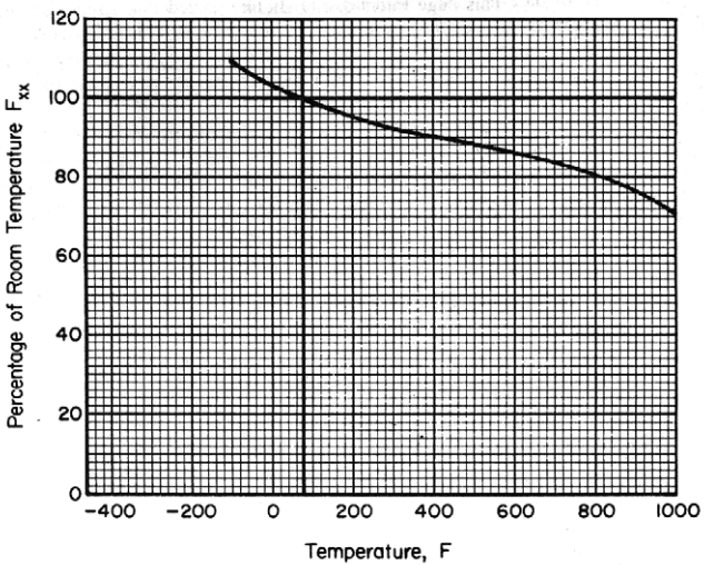
Figure description:
Percentage of Room Temperature Fxx
Percentage of Room Temperature Fxx vs. Temperature
| Temperature, F | Percentage of Room Temperature Fxx |
|---|---|
| -100 | 110 |
| 0 | 104 |
| 75 | 100 |
| 100 | 99 |
| 200 | 96 |
| 300 | 93 |
| 400 | 91 |
| 500 | 89 |
| 600 | 87 |
| 700 | 84 |
| 800 | 81 |
| 900 | 77 |
| 1000 | 71 |
Notes: The chart shows the relationship between temperature and the percentage of room temperature value for a property Fxx. Room temperature (100% is approximately 75°F. The temperature axis ranges from -400 to 1000, but the data curve is plotted from -100 to 1000.)
Figure 9.9.6.3. Typical effect of temperature presentation.
9.9.6.4
Use of Design Data — In footnotes to coupon-derived design data, it is necessary to present precautionary notes on the use of data in structural design. It is recognized that structures may not fail under load in the same manner as a coupon. This lack of one-to-one correlation may be due to differences either in weldment character resulting from potentially higher variability of production welding, or state of stress. Coupon-structure ratios are used to account for these differences.
The coupon-derived basic weld allowable accounts for a sizeable portion of the variability in welded joints; coupon-structure ratio accounts for the remainder. Since the state of stress (and to some extent, distribution of stress) is accounted for in the coupon-structure ratio, it is probable that each general structural configuration will have a unique coupon-structure ratio. For example, the coupon-structure ratio for a tank which must resist internal pressure would be different from the ratio for a welded joint in a sandwich panel.