Proposals presented to the MIL-HDBK-5 Coordination Group should include (1) new or revised table of room-temperature allowables, (2) raw data used in the analysis, and (3) supporting analysis for the proposed design values.
9.8.1
DIRECT ANALYSES OF MECHANICAL PROPERTIES — Computational procedures described in earlier sections are demonstrated here. Several hypothetical sets of input data were created for these example problems. These datasets were created to represent quality assurance test data, representing one long transverse tensile test per lot, plus other tests from a portion of the lots, at a frequency of one test per lot.
The example problems fall into two major categories. Problems I through VII illustrate techniques based on an underlying normal distribution. Problems VIII through XII illustrate techniques based on an underlying three-parameter Weibull distribution.
The input data for these example problems are described below. Because entire data sets (as opposed to means and standard deviations) are required for Problems VIII through XII, the data points for groups (1) through (4) and group (6) are listed in Tables 9.8.1(a) through (c).
INFORMATION FOR EXAMPLE PROBLEMS
Material Identification: Alloy X sheet, annealed. Specified Testing Direction: Long Transverse (LT)
Specified Properties:
inch ;
0.126-0.249 inch — .
Available Test Results:
Group (1). 300 observations of TUS(LT) for thickness range 0.020-0.125 inch from Supplier A; no variation with thickness. Go to Problems I, III, VIII, and X.
Group (2). 300 observations of TYS(LT) for thickness range 0.020-0.125 inch from Supplier A; no variation with thickness. Go to Problems II and IX.
Group (3). 30 observations of TUS(LT) for thickness range 0.020-0.125 inch from Supplier B; no variation with thickness. Go to Problems I and VIII.
Group (4). 30 observations of TYS(LT) for thickness range 0.020-0.125 inch from Supplier B; no variation with thickness. Go to Problems II and IX.
Group (5). 100 observations of TUS(LT) for thickness range 0.126-0.249 inch; no variation with thickness. Go to Problems III and X.
Group (6). 30 observations of SUS(LT) for thickness range 0.020-0.249 inch; apparent decrease in SUS(LT) on increasing thickness; observations may be paired with TUS(LT) if desired. Go to Problem VII.
MIL-HDBK-5J
9.8.3
TABULAR DATA PRESENTATION — The proposal for the incorporation of design allowables into MIL-HDBK-5 will contain supporting data and computations for all design properties. Depending on quantity and availability, data may be tabulated, plotted, or referenced (to readily available technical reports, specifications, etc.). Computations should indicate adequately the manner in which design values were computed and will be presented in an orderly manner. Data sources will be identified.
All minimum mechanical property data analyses must be performed in English units. Strength data recorded in metric units should be converted to English units, to the nearest 0.01 ksi, before data analyses are undertaken. If desired by the data supplier, metric equivalent tables and figures can be included as part of the working data submitted with a data proposal, but the tables and/or figures proposed for inclusion in MIL-HDBK-5 will contain only English units.
9.8.3.1
Mechanical Properties — The table of room-temperature design values will be presented in the format indicated in Figure 9.8.3.1(a) for conventional metallic materials. This format has been designed to accommodate most of these materials; however, some modifications may be required. For example, the format shown in Figure 9.8.3.1(b) will be used for aluminum alloy sheet laminates which are generally anisotropic and have limited ductility. Design values for these hybrid materials are presented for several mechanical properties which differ from those shown for conventional metallic materials. Unused lines (for example, ST properties for sheet) are deleted. Guidance in the use of these formats may be obtained by examining tables throughout this document and by referral to the applicable procurement specification. The following instructions should be followed for the items located in Figure 9.8.3.1(a):
- (1) Table number: If this is a revision of an existing table, use the same table number; otherwise, use a new table number in the proper sequence.
- (2) Material designation: Use a numeric designation where available (for example, 7075 aluminum alloy). Avoid the use of trade names. Include products following the material designation, except products may be omitted from the title if there are many products covered by the table.
- (3) Specification: Refer to a public specification (industry, Military, or Federal), followed by a type or class designation, if appropriate. Do not refer to proprietary specifications.
MIL-HDBK-5J
9.8.3.2
Modulus of Elasticity and Poisson's Ratio — The following room-temperature elasticity values are presented in the room-temperature property tables as typical values:
| Property | Units | Symbol | Recommended ASTM Test Procedures |
|---|---|---|---|
| Modulus of Elasticity | |||
| In tension | 1000 ksi | E | E 111 |
| In compression | 1000 ksi | Ec | E 111 |
| In shear | 1000 ksi | G | E 143 |
| Poisson’s Ratio | (Dimensionless) | μ | E 132 |
If the material is not isotropic, the applicable test direction must be specified. Deviations from isotropy must be suspected if the experimentally determined Poisson’s ratio differs from the value computed by the formula
[9.8.3.2(a)]
where is the average of and .
Given , and may be computed by this equation. Likewise, given , and may be computed from the equation:
[9.8.3.2(b)]
In the event is not available, may be substituted for in the above equations to provide an estimate of either or .
9.8.3.3
Physical Properties — Density, specific heat, thermal conductivity, and mean coefficient of thermal expansion are physical properties normally included in MIL-HDBK-5. Physical properties are presented in the room-temperature property table if they are not presented in effect-of-temperature curves. The basis for physical properties is “typical”. Table 9.8.3.3 displays units and symbols used in MIL-HDBK-5, and also recommended ASTM test procedures for measuring these properties. Since modifications of procedures are employed in measuring physical properties, methods used for values proposed for inclusion in MIL-HDBK-5 should be reported in the supporting data proposal. For specific heat and thermal conductivity values reported in the room temperature property table, the reference temperature of measurement is also shown [for example, for 2017 aluminum the specific heat is 0.23 (at 212°F)]. For tabulated values of mean thermal expansion, temperature range of the coefficient is shown [for example,
MIL-HDBK-5J
9.8.5
ELEVATED TEMPERATURE GRAPHICAL MECHANICAL PROPERTIES — Effects of temperature and of thermal exposure on strength and certain other properties are presented graphically. Methods for determining these curves differ and are described below.
9.8.5.1
Strength Properties — Tensile ultimate and yield strengths, compressive yield strength, shear ultimate strength, and bearing ultimate and yield strengths at temperatures other than room temperature (80 °F) are shown as percentages of room-temperature value for that property. Use of percentage curves allows a single curve to be used in place of multiple curves when more than one room-temperature value is presented for a property, as for example, differing A- and B-design values for each of several thickness ranges. In instances where related properties differ in their response to temperature, additional curves are provided and are labeled to indicate specific properties and forms to which they apply.
No significance level is attached to these curves. For practical purposes, however, the product of a room-temperature A or B design value and an appropriate percentage value from the curve may be regarded as an A or B design value at the indicated temperature.
9.8.5.1.1
Determination of Working Curves — Working curves for each product form, heat treat condition, property, and grain direction should be constructed. Separate curves should be examined to determine if certain data can be combined. For example, it may be possible to combine data for sheet and plate, T73 and T7351 tempers, tensile and compressive yield strengths, or longitudinal and long transverse grain directions.
MIL-HDBK-5J
9.8.5.1.2
Preparation of Finished Curves — When two or more working curves are to be combined into a single curve, percentages shown in the finished curve will represent the separate bound of all individual working curves used in its preparation. When corresponding working curves differ substantially in shape or scaling, it may be appropriate to prepare more than one finished curve (for example, separate curves for longitudinal and transverse testing directions). Finished curves will not exhibit “humps”, such as might appear with a temperature range where aging takes place. Where such humps appear in working curves, these will be leveled by means of horizontal line segments.
MIL-HDBK-5J
31 January 2003
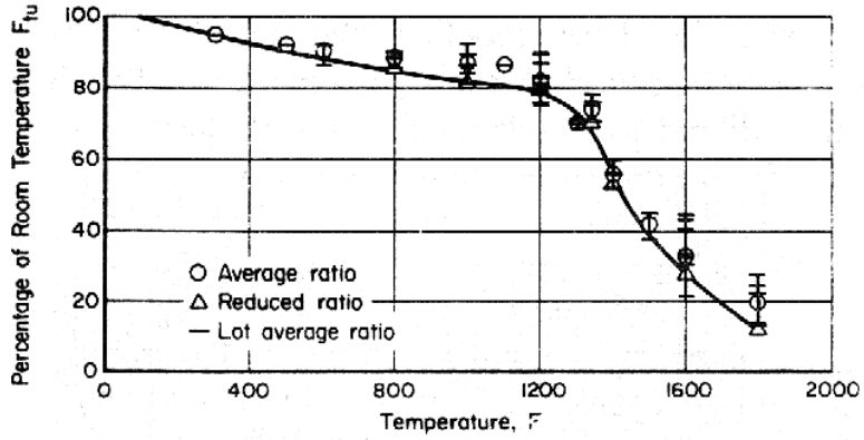
Figure description:
Effect of Temperature on Room Temperature Strength F_tuRatio
Percentage of Room Temperature F_tu vs Temperature
Legend
- Average ratio — color: black; symbol: Circle (o
- Reduced ratio — color: black; symbol: Triangle (Δ
- Lot average ratio — color: black; symbol: Horizontal tick (-
| Temperature, F | Average ratio (o) | Reduced ratio (Δ) | Lot Range (Min) | Lot Range (Max) | Solid line |
|---|---|---|---|---|---|
| 0 | 100 | ||||
| 300 | 95 | 94 | |||
| 500 | 92 | 91 | 89 | 93 | 91 |
| 600 | 90 | 88 | 86 | 91 | 89 |
| 800 | 89 | 86 | 84 | 91 | 84 |
| 1000 | 88 | 82 | 80 | 92 | 82 |
| 1100 | 87 | 81 | |||
| 1200 | 83 | 79 | 75 | 90 | 79 |
| 1300 | 71 | 71 | 69 | 72 | 73 |
| 1350 | 74 | 72 | 69 | 78 | 65 |
| 1400 | 57 | 54 | 53 | 60 | 54 |
| 1500 | 42 | 41 | 38 | 45 | 40 |
| 1600 | 33 | 28 | 21 | 45 | 28 |
| 1800 | 20 | 13 | 15 | 28 | 13 |
Figure 9.8.5.1.1. Working curve drawn through reduced ratios converted to percentages.
Finished curves will be drawn in reproducible form on grids of 10 lines to the inch, with each tenth line accented. The ordinate will normally be scaled in units of 20 percent per inch and will be labeled “Percentage of Room Temperature Strength”. Abscissa will be scaled in units of 100, 200, or 400°F per inch, as appropriate, and will be labeled “Temperature, °F”. Both axes will be annotated at intervals of 1 inch. Not more than two curves will be drawn in a single figure, and these should be labeled clearly to distinguish between them. In addition, each figure will carry a legend containing the words “strength at temperature”, together with exposure limits and other information that would limit the applicability of the curve.
An example of the finished percentage curve is shown in Figure 9.8.5.1.2(a). When practical, single percentage curves, representing and may be located on a single illustration as shown in Figure 9.8.5.1.2(b). Likewise, single curves representative of and may be located on one illustration and curves for and may also be placed on a single illustration.
9.8.5.2
Elongation and Reduction of Area — Elongation and reduction of area are presented as “typical” values at each temperature. If ductility values follow a log-normal distribution, they should be converted to logarithms before averaging. In most cases, the median (middle-most value) will be nearly identical to the average determined in this manner. Ductility values are not converted to percentages of the room-temperature value. Hence, a best smooth curve drawn through the typical values at each temperature is merely redrawn without data points for presentation in the document, as shown in Figure 9.8.5.2. Separate curves may be required for products differing in ductility.
As with strength data, care must be taken to avoid biasing the curve by the inclusion of large quantities of data from some lots and small quantities from others. Use of lot-average values in place of individual measurements is highly recommended.
MIL-HDBK-5J
9.8.5.3
Modulus of Elasticity — The elastic modulus may vary with test direction and product form. Data should be examined before plotting, and if differences are observed, separate working curves should be prepared for each variable. The percentage curve for modulus of elasticity is a best-fit smooth curve drawn through the average of all percentages at each temperature, where individual percentage values are obtained as described in Section 9.8.5.1.1. As with strength data, temperatures should be so selected that the shape of the curve is defined adequately. Figure 9.8.5.3 illustrates a finished percentage curve representing two moduli, and , for which working curves were similar enough to permit their combination into a single curve.
9.8.5.4
Physical Properties — When data are adequate to present curves showing specific heat,
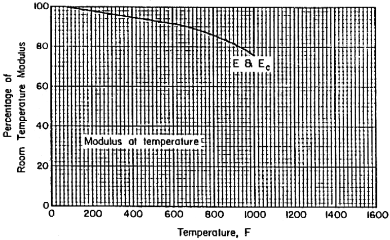
Figure description:
Modulus at Temperature
Percentage of Room Temperature Modulus vs. Temperature
Annotations
- E & E_c (text_label - position: x = 1000, y = 75)
- Modulus at temperature (text_label - position: x = 400, y = 35)
| Temperature, F | Percentage of Room Temperature Modulus (E & E_c) |
|---|---|
| 0 | 100.0 |
| 100 | 98.5 |
| 200 | 97.0 |
| 300 | 95.5 |
| 400 | 94.0 |
| 500 | 92.5 |
| 600 | 91.0 |
| 700 | 88.5 |
| 800 | 86.0 |
| 900 | 81.5 |
| 1000 | 75.0 |
Notes: The chart shows the degradation of the modulus of elasticity (E & Ec as temperature increases. The values are expressed as a percentage of the modulus at room temperature.)
Figure 9.8.5.3. Percentage curve representing two elastic moduli.
MIL-HDBK-5J
9.8.5.5
Effect of Thermal Exposure on Room Temperature Strength — Curves described in this section are presented (1) when the material exhibits a decrease in room-temperature strength as a result of unstressed exposure to elevated temperatures, and (2) when data are not presented in the form of parametric curves (see “Complex-Exposure” in Section 9.8.5.8). Supporting data expressed as percentages of the “no-exposure” strength are plotted with percent of room-temperature strength as the ordinate and exposure temperature as the abscissa. Separate plots are required for each exposure time. Typical exposure times are , and 1000 hours. Design curves are drawn in the same manner as for effect of temperature on strength; humps that may appear in the design curve should be leveled off in drawing the final curve.
The following restrictions are placed on effect-of-exposure curves for strength properties at room temperature:
- (1) Percentage curves for a designated exposure temperature may not show increasing percentage values with increasing exposure time.
- (2) Percentage curves for a designated exposure time may not show increasing percentage values with increasing exposure temperature.
A typical effect-of-exposure curve is illustrated in Figure 9.8.5.5.
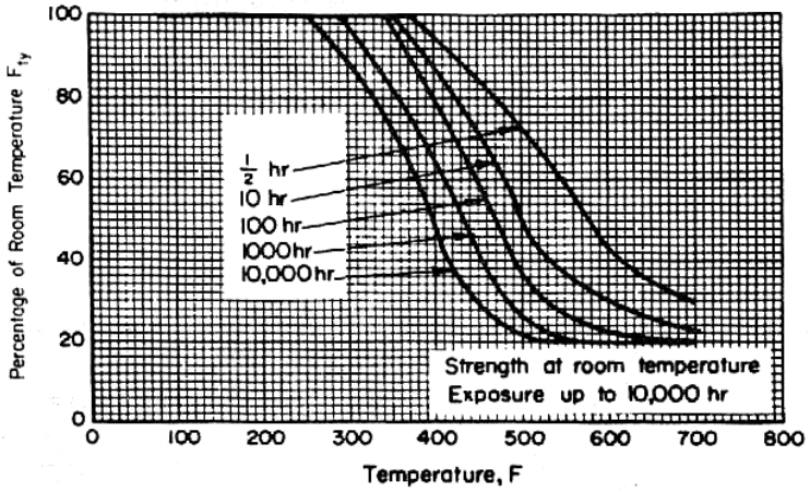
Figure description:
Effect of Temperature and Exposure Time on Yield Strength (Fty Retention
Percentage of Room Temperature Fty vs. Temperature, F
Legend
- 1/2 hr — color: black; symbol: solid line
- 10 hr — color: black; symbol: solid line
- 100 hr — color: black; symbol: solid line
- 1000 hr — color: black; symbol: solid line
- 10,000 hr — color: black; symbol: solid line
Annotations
- Strength at room temperature Exposure up to 10,000 hr (text_label - position: bottom-right corner of the grid)
| Temperature (F) | 1/2 hr | 10 hr | 100 hr | 1000 hr | 10,000 hr |
|---|---|---|---|---|---|
| 0 | 100 | 100 | 100 | 100 | 100 |
| 100 | 100 | 100 | 100 | 100 | 100 |
| 200 | 100 | 100 | 100 | 100 | 100 |
| 230 | 100 | 100 | 100 | 100 | 100 |
| 250 | 100 | 100 | 100 | 100 | 92 |
| 280 | 100 | 100 | 100 | 92 | 82 |
| 300 | 100 | 100 | 96 | 84 | 74 |
| 350 | 100 | 92 | 80 | 64 | 50 |
| 400 | 96 | 78 | 58 | 40 | 30 |
| 450 | 82 | 56 | 36 | 24 | 20 |
| 500 | 60 | 38 | 24 | 18 | 16 |
| 550 | 48 | 30 | 20 | null | null |
| 600 | 38 | 26 | 18 | null | null |
| 650 | 32 | 24 | null | null | null |
| 700 | 30 | 22 | null | null | null |
Figure 9.8.5.5. Effect of exposure at elevated temperatures on room-temperature properties.
9.8.5.6
Effect of Thermal Exposure on Elevated Temperature Strength — The effect of thermal exposure on elevated-temperature strength is presented in one of two manners, depending upon whether or not the exposure temperature equals the test temperature. In the case of simple exposure, exposure temperature and test temperature are assumed to be identical. For complex exposure, exposure temperature and test temperature need not be the same. When either of these curves is presented in MIL-HDBK-5, it includes all information normally presented in elevated temperature curves described in Section 9.8.5.1; thus, these curves replace the elevated temperature curves.
MIL-HDBK-5J
9.8.5.7
Simple Exposure — The curves are prepared in the same manner as basic elevated temperature curves described in Section 9.8.5.1. Separate design curves are prepared for each exposure time, and presented in a single figure. Typical exposure times for the curves are ½, 10, 100, and 1000 hours.
The following additional restrictions are placed on effect-of-exposure curves for strength properties at elevated temperatures:
- (1) Percentage curves for a designated exposure (test) temperature may not show increasing percentage values with increasing exposure time.
- (2) Percentage curves for a designated exposure time may not show increasing percentage values with increasing exposure (test) temperature.
A typical set of curves for exposure at test temperature is illustrated in Figure 9.8.5.7.
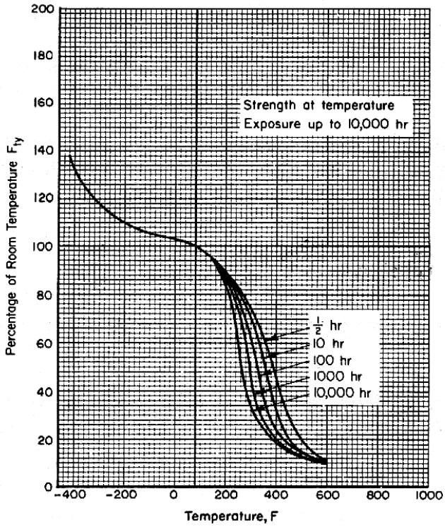
Figure description:
Strength at Temperature for Exposure up to 10,000 hr
Percentage of Room Temperature Fty vs. Temperature, F
Legend
- 1/2 hr — color: black; symbol: Solid line
- 10 hr — color: black; symbol: Solid line
- 100 hr — color: black; symbol: Solid line
- 1000 hr — color: black; symbol: Solid line
- 10,000 hr — color: black; symbol: Solid line
Annotations
- Strength at temperature Exposure up to 10,000 hr (text_label - position: x = 650, y = 160)
| Temperature (F) | 1/2 hr (%) | 10 hr (%) | 100 hr (%) | 1000 hr (%) | 10,000 hr (%) |
|---|---|---|---|---|---|
| -400 | 138 | 138 | 138 | 138 | 138 |
| -300 | 121 | 121 | 121 | 121 | 121 |
| -200 | 110 | 110 | 110 | 110 | 110 |
| -100 | 105 | 105 | 105 | 105 | 105 |
| 0 | 103 | 103 | 103 | 103 | 103 |
| 75 | 100 | 100 | 100 | 100 | 100 |
| 160 | 96 | 96 | 96 | 96 | 96 |
| 200 | 92 | 92 | 92 | 92 | 92 |
| 240 | 88 | 86 | 82 | 76 | 70 |
| 280 | 82 | 74 | 64 | 52 | 42 |
| 320 | 72 | 61 | 49 | 38 | 30 |
| 360 | 60 | 48 | 36 | 26 | 22 |
| 400 | 48 | 35 | 26 | 19 | 17 |
| 440 | 37 | 26 | 19 | 15 | 14 |
| 480 | 28 | 19 | 15 | 13 | 12 |
| 520 | 21 | 15 | 13 | 12 | 11 |
| 600 | 14 | 12 | 11 | 11 | 11 |
Figure 9.8.5.7. Simple-exposure curves.
MIL-HDBK-5J
9.8.5.8
Complex Exposure — In these curves, thermal-exposure variables, time, and temperature are combined into an exposure parameter, which is plotted as the abscissa. The ordinate is expressed in the same manner as in effect-of-temperature curves. Separate percentage curves are presented for each test temperature. In addition, each figure contains a nomograph for use in converting exposure time and temperature to the exposure parameter.
The exposure parameter may be of the form , where is exposure temperature in degrees F, C is a constant, and t is exposure time in hours. There are a number of ways to determine the values of C. The simplest method is to select (by interpolation of test data) two exposure conditions that produce the same strength at some designated test temperature, set two parameters equal to each other, and solve for C. For example, assume that the following data are obtained:
| Exposure | TUS at 400 °F, ksi | |
|---|---|---|
| Time, hr | Temp, °F | |
| 1000 | 400 | 80.0 |
| 1 | 500 | 83.0 |
| 10 | 500 | 78.0 |
Plot 500°F data as stress versus log time; a straight line between (83, log 1) and (78, log 10) crosses 80 ksi at log 4 (hours). Thus, 4 hours' exposure at 500°F is equal to 1000 hours' exposure at 400°F:
,
C = 20.
This exercise should be repeated for several pairs of exposure conditions to obtain an average value for C.
Alternatively, several equivalent exposure conditions may be plotted as log exposure time (ordinate) versus 1/(T F + 460) (abscissa). A best-fit straight line is drawn through the plotted points and its slope determined. C is then found from the relationship
C = m/(T F + 460) - log t,
where is slope and and are coordinates of any point on the line. This method is amenable to data-regression procedures described in Section 9.5.6, from which a least-squares estimate of C is obtained. Separate data plots are prepared for each test temperature, using percent of "no-exposure" room-temperature strength as the ordinate, and as the abscissa. Design curves are then drawn as described in Section 9.8.5.1.1.
A typical complex-exposure curve is illustrated in Figure 9.8.5.8. It should be noted that the abscissa scale is not shown in the figure since the time-temperature nomograph is used directly to locate the position on the abscissa.