9.5analysis procedures for statistically computed minimum static properties

9.5.1.1

Deciding Between Direct and Indirect Computation — The only room-temperature design properties that are regularly determined by direct computation are $F_{t u}$ and $F_{t y}$. This procedure is usually limited to a specified or usual testing direction because there are seldom enough data available to determine properties in other test directions. Two rules govern the choice between direct and indirect computation:

• (1) $F_{t u}$ and $F_{t y}$ in the specified or usual testing direction may be determined by direct computation only.
• (2) $F_{t u}$ and $F_{t y}$ in other testing directions (as well as $F_{c y}, F_{s u}, F_{b r u}$, and $F_{b r y}$ in all directions) may be determined by direct computation only if (a) the data are adequate to determine the distribution form and reliable estimates of population parameters, or (b) the sample includes 299 or more individual, representative observations of the property to be determined.

MIL-HDBK-5J

9.5.1.2

Testing for Regression Effects and Homogeneity — In most cases, there will be a fairly clear-cut division between one population and another. For example, L and T properties either are or are not nearly identical. However, wrought product properties may sometimes vary linearly or curvilinearly with some dimensional characteristic, such as thickness. Examples are effect of thickness on TUS, effect of temperature on TUS, and effect of stress on cycles or time to rupture. It is necessary, therefore, to first test the data for the relationship between the property and the material dimension.

Before employing a regression analysis in the determination of material properties, one must ascertain that the average of the property to be regressed varies continuously and linearly or quadratically with some dimensional parameter x (such as x = t, 1/t, etc., where t is thickness). If the variation of average is attributable to other causes, regression should not be used.

Regression analysis, as described herein, also assumes that residuals are normally distributed about the regression line. Residuals are the differences between observed data values and the values which are predicted by the fitted regression equation. Validity of this normality assumption should be evaluated by performing the Anderson-Darling test presented in Section 9.5.4.1.

The procedures for fitting a regression equation of the form,

to n data points are described in Section.9.5.2. In addition to estimates for a and b (and possibly c), this procedure produces two F statistics. One statistic ( $\mathrm{F}_{1}$ ) tests the significance of regression. The other statistic $\left(\mathrm{F}_{2}\right)$ tests the adequacy of a linear model for describing the relationship between the material property and the dimensional parameter. If $\mathrm{F}_{2}$ indicates a lack of fit of the model to the data, a transformation of the data may account for the nonlinearity. If $\mathrm{F}_{1}$ indicates an insignificant regression, one of the other appropriate analysis techniques, as described in Section 9.5.5 for direct computation, or 9.5.7 for indirect computaion, should be used.

MIL-HDBK-5J

MIL-HDBK-5J

9.5.2.1

Linear Regression — Linear regression is appropriate when there is an approximate linear relationship between two measurable characteristics. Such a relationship is expressed algebraically by an equation that, in the case of two measurable characteristics x and y, has the form

[9.5.2.1(a)]

where x = independent variable y = dependent variable $\alpha$ = true intercept of the regression equation $\beta$ = true slope of the regression equation $\varepsilon$ = measurement or experimental error by which y differs from the ideal linear relationship.

Aside from the error term, ε, this is the equation of a straight line. The parameter α determines the point where this line intersects the y-axis, and the β represents its slope. The variables x and y may represent either direct measurements or some transformation measurements of the characteristics under consideration.

Knowing or assuming such an approximate linear relationship, the problem becomes one of estimating the parameters $\alpha$ and $\beta$ of the regression equations. It is necessary to have a random sample consisting of n pairs of observations, which is denoted by $\left(\mathrm{x}_{1}, \mathrm{y}_{1}\right),\left(\mathrm{x}_{2}, \mathrm{y}_{2}\right), \ldots,\left(\mathrm{x}_{\mathrm{n}}, \mathrm{y}_{\mathrm{n}}\right)$. Such a sample can be represented graphically by n points plotted on a coordinate system, in which x is plotted horizontally and y vertically. A subjective solution can be obtained by drawing a line that, by visual inspection, appears to fit the points satisfactorily. An objective solution is given by the method of least squares.

The method of least squares is a numerical procedure for obtaining a line having the property that the sum of squares of vertical deviations of the sample points from this line is less than that for any other line. In this analysis, the least-squares line is represented by the equation

[9.5.2.1(b)]

in which

ŷ = predicted value of y for any value of x

a and b = estimates of the parameters $\alpha$ and $\beta$ in the true regression equation obtained by the least squares method presented below.

MIL-HDBK-5J

9.5.2.2

Quadratic Regression — Quadratic regression is appropriate when there is an approximate quadratic relationship between two measurable characteristics. Such a relationship is expressed algebraically by an equation that, in the case of two measurable characteristics x and y, has the form

[9.5.2.2(a)]

MIL-HDBK-5J

31 January 2003

where

x: independent variable y: dependent variable

Aside from the error term, ε, this is the equation of a parabola. The parameter α determines the point where this curve intersects the y-axis. The variable x and y may represent either direct measurements or some transformation measurements of the characteristics under consideration.

Knowing or assuming such an approximately quadratic relationship, the problem becomes one of estimating the parameters $\alpha, \beta$, and $\gamma$ of the regression equation. It is necessary to have a random sample consisting of n pairs of observations, which is denoted by $\left(\mathrm{x}_{1}, \mathrm{y}_{1}\right),\left(\mathrm{x}_{2}, \mathrm{y}_{2}\right), \ldots,\left(\mathrm{x}_{\mathrm{n}}, \mathrm{y}_{\mathrm{n}}\right)$. Such a sample can be represented graphically by n points plotted on a coordinate system, in which x is plotted horizontally, y vertically. A subjective solution can be obtained by drawing a curve that, by visual inspection, appears to fit the points satisfactorily. An objective solution is given by the method of least squares.

The method of least squares is a numerical procedure for obtaining a second-degree polynomial having the property that the sum of squares of vertical deviations of the sample points from this curve is less than that for any other second-degree polynomial. In this analysis, the least squares curve is represented by the equation

$\hat{\mathrm{y}}\ =\ \mathrm{a}\ +\ \mathrm{bx}\ +\ \mathrm{cx}^2\ \ ,$ [9.5.2.2(b)]

in which

$\hat{\text{y}}=$: predicted value of y for any value of x a, b, and c =: estimates of the parameters $\alpha$, $\beta$ and $\gamma$ in the true regression equation obtained by the least squares method presented below.

It can be shown with the aid of calculus that the values of a, b, and c that minimize the sum of squares of the vertical deviations are given by the formulas:

$a = \overline {y} - b\left( \sum \frac {x} {n}\right) - c\left( \sum \frac {x^{2}} {n}\right)$ $b = \frac {(\sum X_{1}Y)(\sum X_{2}^{2}) - (\sum X_{2}Y)(\sum X_{1}X_{2})} {D}$

$c = \frac{(\sum X_2 Y)(\sum X_1^2) - (\sum X_1 Y)(\sum X_1 X_2)}{D}$ [9.5.2.2(c)]

9.5.2.3

Tests for Adequacy of a Regression — It is possible that the relationship between the dependent variable y and the independent variable x may not be well approximated by the chosen model (linear or quadratic). In that case, the predicted values, modeled by a line or a quadratic curve, would not “fit” the data very well. It is also possible that the relationship between x and y, although well described by the chosen model, is not very strong. That is, there may not be much change in the y values over the range of x considered. This is measured by the “significance” of the regression. Both the lack of fit and the significance of a linear regression equation can be evaluated through an analysis of variance as described in this section.

To evaluate the adequacy of a regression model requires satisfying two conditions. First, it is necessary that there are multiple observations at one or more values of the independent variable x. Second, in the case of a linear regression, there must be three or more distinct x values; in the case of a quadratic regression, there must be four or more distinct x values.

The analysis of variance for testing lack of fit and significance of regression is based on the assumption that the measurement errors, $\varepsilon_{\mathrm{i}}$, in the relationship between $y_{\mathrm{i}}$ and $x_{\mathrm{i}}$ [see 9.5.2.1(a) and 9.5.2.2(a)] are independent and normally distributed with an overall mean of zero and a constant variance of $\sigma^{2}$. Assuming uniformity of variance of measurement errors over the range of the independent variable, the normality assumption concerning unobservable $\varepsilon_{\mathrm{i}}$ can be checked by performing the Anderson-Darling test for normality on the observed residuals

$\mathbf{e}_{\mathrm{i}}=y_{\mathrm{i}}-\hat{y}_{\mathrm{i}}$,

i=1,..., n, where

ŷ_i=a+bx_i

of the inverted matrix $\left(X^{\prime} X\right)^{-1}=\left[\begin{array}{ccc}q_{1} & q_{2} & q_{3} \\ q_{2} & q_{4} & q_{5} \\ q_{3} & q_{5} & q_{6}\end{array}\right]$, where $X^{\prime} X=\left[\begin{array}{cc}n & \sum x_{i} \\ \sum x_{i} & \sum x_{i}^{2} \\ \sum x_{i}^{2} & \sum x_{i}^{3}\end{array}\right]$

MIL-HDBK-5J

31 January 2003

in the case of linear regression, and

$\hat{y}_{\mathrm{i}}=\mathrm{a}+\mathrm{b} x_{\mathrm{i}}+\mathrm{c} x_{\mathrm{i}}^{2}$

in the case of quadratic regression. See Sections 9.5.2.1 and 9.5.2.2 for details on the computation of a, b, and c, and see Section 9.5.4.1 for details on the Anderson-Darling test for normality. By plotting the residuals, $\mathrm{e}_{\mathrm{i}}$, against the respective $\mathrm{x}_{\mathrm{i}}$, an informal check on the assumption of constant variance is possible as well. In such a plot, residuals should vary approximately equally over the range of $\mathrm{x}_{\mathrm{i}}$ values.

The analysis of variance table for testing lack of fit and significance of a linear regression is shown below. In this table, n represents the total number of data points for which x and y are available, k represents the number of distinct x values. Formulas for calculating the terms provided in the table are described below.

The sums of squares (SS terms) for the Regression, Error, and Total lines of the analysis of variance table are calculated using the following:

$\begin{aligned} S S R & =\sum\left(\hat{y}_{i}-\overline{y}\right)^{2} \\ S S T & =\sum\left(y_{i}-\overline{y}\right)^{2} \\ S S E & =\sum\left(y_{i}-\hat{y_{i}}\right)^{2}\end{aligned}$

To calculate the sums of squares for lack of fit (SSLF) and pure error (SSPE) requires a relabeling of the data, ordered by x value. To this point, the measured values $y_{\mathrm{i}}$ have been arbitrarily ordered. For these calculations, let $Y_{\mathrm{u} j}$ represent the j $\mathrm{th}$ data value at the $\mathrm{u}^{\text {th }} \mathrm{x}$ level, and let $\mathrm{n}_{\mathrm{u}}$ represent the number of data values at the $\mathrm{u}^{\text {th }} \mathrm{x}$ level. Let

$\overline{\mathrm{Y}}_{\mathrm{u}}=\sum_{\mathrm{j}=1}^{\mathrm{n}_{\mathrm{u}}} \mathrm{Y}_{\mathrm{uj}} / \mathrm{n}_{\mathrm{u}}$

MIL-HDBK-5J

9.5.2.4

Testing for Equality of Several Regressions — The procedure presented in this section is designed to test the hypothesis that the true regression equations corresponding to two or more independent data sets are equal (linear or quadratic). It is appropriately applied to test the equality of several regressions in determining whether corresponding data sets should be combined for the purpose of calculating design allowables. To test k regressions for equality, the following procedure should be performed.

Perform separate regression analyses for each data set. The same model form should be used in all regressions (all linear or all quadratic). Add error sum of squares (SSE) values from each of the separate regressions to obtain SSE(F), the error sum of squares for the full model which allows separate slope and intercept parameters for each data set. Then fit a single regression to the combined data from all data sets to obtain SSE(R), error sum of squares for the reduced model which contains a single set of coefficients a and b (and c for quadratic models) which apply to all data sets. The F statistic for testing the equality of the k regressions is

$\mathrm{F}=\frac{\mathrm{SSE}(\mathrm{R})-\mathrm{SSE}(\mathrm{F})}{2(\mathrm{k}-1)} \div \frac{\mathrm{SSE}(\mathrm{F})}{\mathrm{n}-2 \mathrm{k}}$

for simple linear models, and

$\mathrm{F}=\frac{\mathrm{SSE}(\mathrm{R})-\mathrm{SSE}(\mathrm{F})}{3(\mathrm{k}-1)} \div \frac{\mathrm{SSE}(\mathrm{F})}{\mathrm{n}-3 \mathrm{k}}$

for quadratic models, where n denotes total number of observations in all k data sets combined. In the linear case, if F is greater than the 95th percentile of the F distribution with 2(k - 1) numerator degrees of freedom and n - 2k denominator degrees of freedom (from Table 9.10.2), the hypothesis that the regressions are equal is rejected. In the quadratic case, if F is greater than the 95th percentile of the F distribution with 3(k - 1) numerator degrees of freedom, and n - 3k denominator degrees of freedom, the hypothesis that the regressions are equal is rejected. See Reference 9.5.2.4 for more detail.

Example of Computations — In this example, x represents thickness and y represents the TYS values determined from a group of tensile tests. Values of x and y are as follows:

MIL-HDBK-5J

9.5.3.1

The k-Sample Anderson-Darling Test — The k-sample Anderson-Darling test is designed to test the hypothesis that populations from which two or more independent random samples were drawn are identical. The test is appropriately applied to determine whether two or more products differ with regard to strength distributions. The test is a nonparametric statistical procedure and, thus, requires no assumptions other than the samples are true independent random samples from their respective populations.

MIL-HDBK-5J

9.5.3.2

The F Test — The F test is used to determine whether the strength of two products differs with regard to variability.

Consider two products, A and B. These might represent two different processes, thickness ranges, or test directions. The statistics for the samples drawn from these products are:

F is the ratio of the two sample variances, thus,

[9.5.3.2]

If the true variances of Products A and B are identical at a significance level of $\alpha=0.05$, F should lie within the interval defined by

$\mathrm{F}_{0.975}$ (for $\mathrm{n}_{\mathrm{A}}-1$ and $\mathrm{n}_{\mathrm{B}}-1$ degrees of freedom),

and

$1 / \mathrm{F}_{0.975}$ (for $\mathrm{n}_{\mathrm{B}}-1$ and $\mathrm{n}_{\mathrm{A}}-1$ degrees for freedom). *

If F does not lie within this interval, it can be concluded that the two products differ with regard to their variability. Values of $\mathrm{F}_{0.975}$ are presented in Table 9.10.3.

MIL-HDBK-5J

9.5.3.3

The t Test — The t test is used to determine whether two products differ with regard to average strength. If they do, one may conclude that the two products do not belong to the same population.

In making the t test, it is assumed that the variances of two products are nearly equal, as first determined from the F test. If the F test shows that the variances are significantly different, there is no need to conduct the t test.

Consider the same products, A and B. The statistics for samples drawn from these products are:

$\mathrm{D}_{\mathrm{x}}$ is the absolute difference between the two sample means.

[9.5.3.3(a)]

If the true means of products A and B are identical, $\mathrm{D}_{\mathrm{x}}$ should not exceed u, which is determined as indicated by the following equation for a significance level of $\alpha=0.05$.

$u=t_{0.975}s_{p}\sqrt{\frac{n_{A}+n_{B}}{n_{A}n_{B}}}$ [9.5.3.3(b)]

MIL-HDBK-5J

9.5.4.1

"Anderson-Darling" Test for Normality — The "Anderson-Darling" test for normality is used to determine whether the curve which fits a given set of data can be approximated by a normal curve. The essence of the test is a numerical comparison of the cumulative distribution function for observed data with that for the fitted normal curve over the entire range of the property being measured. Let

$\mathrm{Z}_{(\mathrm{i})}=\left(\mathrm{X}_{(\mathrm{i})}-\overline{\mathrm{X}}\right) / \mathrm{s} \quad \mathrm{i}=1, \ldots, \mathrm{n}$

where $X_{(\mathrm{i})}$ is the $\mathrm{i}^{\text {th }}$ smallest sample observation, $\overline{\mathrm{X}}$ is the sample average, and s is the sample standard deviation. Equations for computing sample statistics are presented in Appendix A.

The "Anderson-Darling" test statistic is

where $\mathrm{F}_{\mathrm{o}}$ is the standard normal distribution function*. If

$\mathrm{AD}>0.752 /\left(1+0.75 / \mathrm{n}+2.25 / \mathrm{n}^{2}\right)$

MIL-HDBK-5J

9.5.4.2

Normal Probability Plot —To graphically illustrate the degree to which a normal distribution fits a set of data, a normal probability plot may be formed by plotting the measured value of each test point versus $\overline{\mathrm{X}}+\mathrm{s} \mathrm{F}_{\mathrm{o}}{ }^{-1}(\mathrm{P} / 100)$ where $\mathrm{F}_{\mathrm{o}}{ }^{-1}$ is the inverse standard normal cumulative distribution function.* The line representing the fitted normal distribution is the line passing through the points with equal horizontal and vertical coordinates. If the horizontal axis is labeled with cumulative probabilities (P values) as in Table 9.10.5 rather than $\mathrm{F}_{\mathrm{o}}{ }^{-1}(\mathrm{P} / 100)$ values, the plot will be identical to a plot formed on normal probability paper.

Figure 9.5.4.2 illustrates the use of a normal probability plot on Alclad 2524-T3 Aluminum Alloy Sheet and Plate data in the 0.063-0.128 inch thickness range. There are 309 measured test values with $\overline{\mathrm{X}}$ $=45.24$ and $\mathrm{s}=1.923$. There appears to be a systematic departure from the model (the measured values are higher than expected) in both tails, suggesting that the distribution of the measured values departs from a normal distribution. This model was rejected by the Anderson-Darling test for normality.

9.5.4.3

Three-Parameter Weibull Acceptability Test — The three-parameter Weibull acceptability test is designed to determine whether an acceptable proportion of a producer’s population is likely to exceed the specification limit for corresponding material property. Because this test is only used to screen data sets and is not used in the actual calculation of lower tolerance bounds, it is not required that the data be well-described by a Weibull distribution to apply this test. To carry out this test, an upper confidence bound (UCB) is calculated for the first percentile of the producer’s population. This UCB value is calculated in the same manner as a $\mathrm{T}_{99}$ value is calculated (in Section 9.5.5.2) with the following modifications:

• (1) In solving for the threshold $\tau(\theta)$ (Section 9.5.5.2.1), $\theta$ should be set equal to 0.10 .
• (2) The value of V99 should be taken from Table 9.10.6 rather than Table 9.10.7 when using the formula for T99 (Equation [ 9.5.5.2(a)]) to calculate the UCB value.

MIL-HDBK-5J

31 January 2003

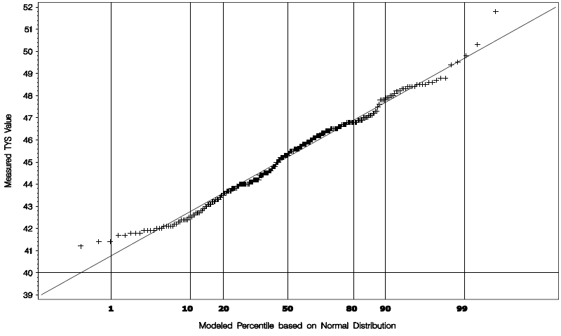
Figure description:

Normal Probability Plot Modeled Percentile based on Normal Distribution vs. Measured TYS Value

Normal Probability Plot of Measured TYS Value

Legend

• Measured TYS Value — color: black; symbol: Cross (+
• Normal Distribution Reference Line — color: black; symbol: Solid line

Annotations

• Grid line at Percentile 1 (vertical_line - position: x = 1)
• Grid line at Percentile 10 (vertical_line - position: x = 10)
• Grid line at Percentile 20 (vertical_line - position: x = 20)
• Grid line at Percentile 50 (vertical_line - position: x = 50)
• Grid line at Percentile 80 (vertical_line - position: x = 80)
• Grid line at Percentile 90 (vertical_line - position: x = 90)
• Grid line at Percentile 99 (vertical_line - position: x = 99)
• Reference line at TYS = 40 (horizontal_line - position: y = 40)

Vertical reference lines plotted at 1st, 10th, 20th, 50th, 80th, 90th, and 99th percentiles of fitted distribution Horizontal reference line plotted at spec minimum, 40 ksi

Figure 9.5.4.2 Probability plot for a normal distribution fitted to a complete TYS data set for Alclad 2524-T3 aluminum alloy sheet in the 0.063-0.128 inch thickness range - rejected.

If UCB is greater than or equal to the specification limit, it is concluded that the producer’s data is acceptable. If UCB is less than the specification limit, it is concluded (with a 5 percent risk of error) that the producer’s data do not meet the specification minimum value.

In statistical terms, this method tests (at 5 percent significance level) the hypothesis that at least 99 percent of the producer’s population is greater than the specification limit. If the hypothesis is not rejected (UCB greater than or equal to specification limit), then it is concluded that the producer’s data is acceptable. If the hypothesis is rejected (UCB less than the specification limit), it is concluded that the producer’s data is unacceptable.

This technique is applicable only when data have not been censored from the sample. It also assumes that the data are distributed according to a three-parameter Weibull distribution (although normally distributed data and Pearson distributed data are also accommodated by this test). If the data sample is highly skewed, background data should be reviewed to determine whether the skewness is caused by a mixed population. If it is not, the Weibull test procedure can be applied. This test should be applied to both tensile yield and ultimate strengths (in appropriate grain directions), and if a producer’s data is unacceptable for either property, that producer’s data for both properties should be excluded for the purpose of computing $\mathrm{T}_{99}$ and $\mathrm{T}_{90}$ values.

9.5.4.4

Anderson-Darling Test for Pearsonality – This section describes a test to determine whether data from a population are satisfactorily described by the Pearson Type III (or gamma) distribution.

MIL-HDBK-5J

9.5.4.5

The Pearson Backoff Option – If the data are rejected by the Pearson AD test, the backoff method may be applied. The following formula should be used to calculate the AD statistic of the backoff method:

$\mathrm{AD}_{\text {backoff }}(\mathbf{u})=\frac{1}{\mathbf{n}} \sum_{\mathbf{i}=1}^{\mathbf{n}} \mathbf{i}^{2}\left[\ln \left(\mathbf{b}_{\mathbf{i}+\mathbf{1}, \mathbf{i}}\right)-\ln \left(\mathbf{b}_{\mathbf{i}, \mathbf{i}}\right)\right]-2 \sum_{\mathbf{i}=1}^{\mathbf{n}} \mathbf{i}\left(\mathbf{b}_{\mathbf{i}+\mathbf{1}, \mathbf{i}}-\mathbf{b}_{\mathbf{i}, \mathbf{i}}\right)+\frac{\mathbf{n}}{2} \sum_{\mathbf{i}=1}^{\mathbf{n}}\left(\mathbf{b}_{\mathbf{i}+\mathbf{1}, \mathbf{i}}^{2}-\mathbf{b}_{\mathbf{i}, \mathbf{i}}^{2}\right)$

MIL-HDBK-5J

9.5.4.6

Pearson Probability Plot — To graphically illustrate the degree to which a Pearson Type III (or gamma) distribution fits a set of data, the following procedure for creation of a Pearson probability plot is recommended. This method is appropriate for distributions estimated using uncensored data.

The rank of each point selected for plotting is the number of lower test points plus the plotted point plus one-half the number of other test points equal to the plotted point. Its cumulative probability, P (in percent), is equal to the rank multiplied by 100, divided by one more than the total number of test points:

P (in percent) = (rank)(100)/n + 1

The measured value of each test point is plotted versus $\mathrm{F}^{-1}(\mathrm{P} / 100)$ where

MIL-HDBK-5J

9.5.4.7

Modified "Anderson-Darling" Test for Weibullness — The "Anderson-Darling" test for three-parameter Weibullness is used to determine whether the curve which fits a given set of data can be approximated by a three-parameter Weibull curve. The essence of the test is a numerical comparison of the cumulative distribution function for observed data with that for a fitted Weibull curve over the entire range of property being measured. This test differs from the original version of the Anderson-Darling test in that it emphasizes the lower tail. This method can be applied with complete or censored data.

The first two steps produce estimates of the parameters of a three-parameter Weibull distribution. Be sure to acknowledge the appropriate degree of censoring in computing the threshold, shape, and scale parameters as described in Sections 9.5.4.7.1 and 9.5.4.7.2. Using the procedure outlined in 9.5.4.7.1, compute the threshold for the goodness-of-fit test, $\tau_{50}$. Then, using the method described in 9.5.4.7.2, compute the maximum likelihood estimates of the shape and scale parameters for $\left\{X_{(i)}-\tau_{50}: i=1, \ldots, r\right\}$ where $r$ equals n for the uncensored data and $r$ represents the smallest integer greater than or equal to $4 n / 5$ for 20 percent censoring and $n / 2$ for 50 percent censoring. Denote these estimates by $\beta_{50}$ and $\alpha_{50}$, respectively. Calculate the (censored or uncensored) A-D statistic is described in Section 9.5.4.7.3.

9.5.4.7.1

Estimating the Threshold Parameter — This section describes a method for estimating the threshold of a three-parameter Weibull distribution. The same approach is taken for estimating the threshold, whether the purpose is to test goodness-of-fit (Section 9.5.4.7), or to directly calculate $\mathrm{T}_{99}$ or $\mathrm{T}_{90}$ values (Section 9.5.5.2). This method applies to uncensored and upper-tail censored data; however, different columns of Table 9.10.8 are used. (References 9.5.4.7.1(a) and 9.5.4.7.1(b) provide details of this method for uncensored data.)

Let K equal the greatest integer less than or equal to min {4n/15, (1-p)n/3}, where p represents the proportion of the upper tail that is censored (p equals 0, 0.2, or 0.5). Define the function R(τ) by

where

with

MIL-HDBK-5J

9.5.4.7.2

Estimating the Shape and Scale Parameters — This section describes a method for estimation of the shape and scale parameters of the two-parameter Weibull distribution based on data which may be censored in the upper tail. Estimates of the shape and scale parameters are based on the original data corrected for the estimated threshold, $\tau$. That is, the calculations in this section are performed based on $Z_{(1)}$, $\ldots, Z_{(n)}$, where $Z_{(\mathrm{i})}=X_{(\mathrm{i})}-\tau$, with $\tau$ estimated as in Section 9.5.4.7.1. The assumption is made here that if the data are censored, then only the $r$ smallest observations in the sample are observed $(1 \leq r \leq n)$, where $r$ is some pre-specified number (often based on a percentage); this is called Type II censoring. Thus, the input to this procedure is a total sample size, $n$, a censored sample size, $r$, and the sample remaining after censoring $Z_{(1)}, \ldots, Z_{(r)}$. Define

$\mathrm{g}(\beta)=\frac{\sum_{\mathrm{i}=1}^{\mathrm{r}} \mathrm{Z}_{(\mathrm{i})}^{\beta} \ln \mathrm{Z}_{(\mathrm{i})}+\left(\mathrm{n}-\mathrm{r}\right) \mathrm{Z}_{(\mathrm{r})}^{\beta} \ln \mathrm{Z}_{(\mathrm{r})}}{\sum_{\mathrm{i}=1}^{\mathrm{r}} \mathrm{Z}_{(\mathrm{i})}^{\beta}+\left(\mathrm{n}-\mathrm{r}\right) \mathrm{Z}_{(\mathrm{r})}^{\beta}}-\frac{1}{\beta}-\frac{1}{r} \sum_{i=1}^{r} \ln Z_{(i)}$

Note: When implementing the equation for g(β) in software, it may be necessary to divide each Z term that is raised to the β power by a normalizing factor, C, in order to avoid computational difficulties. The factor, C, can be any type of average calculated from the Z values (e.g., geometric mean of the uncensored Z values). Because the C-factor algebraically cancels out of the equation for g(β), its use does not change the meaning of the equation in any way.

The shape parameter estimate, $\beta$, is the solution to the equation $g(\beta)=0$. The function $g(\beta)$ is a monotonically increasing continuous function of $\beta$. A simple method for finding the solution is as follows. Let $S_{y}$ denote the standard deviation of $Y_{1}, \ldots, Y_{r}$ where $Y_{i}=\ln \left(Z_{i}\right)$ for $i=1, \ldots, r$. Calculate $I=1.28 / S_{y}$ as an initial guess at the solution and calculate $g(I)$. If $g(I)>0$, then find the smallest positive integer $k$ such that $g\left(I / 2^{k}\right)<0$ and let $L=I / 2^{k}$ and $H=I / 2^{k-1}$. If $g(I)<0$, then find the smallest positive integer $k$ such that $g\left(2^{k} I\right)>0$ and let $L=2^{k-1} I$, and $H=2^{k} I$. Reduce the (L,H) interval by calculating $M=(L+H) / 2$ and setting

MIL-HDBK-5J

9.5.4.7.3

Calculating the Anderson-Darling Statistic — Once the parameters have been estimated in Sections 9.5.4.7.1 and 9.5.4.7.2, calculate the Anderson-Darling statistic by the following steps.

For i=1,...,r, let

$\mathrm{F}_{\mathrm{i}}=1-\exp \left(-\left(\frac{\mathrm{X}_{(\mathrm{i})}^{-\tau_{50}}}{\alpha_{50}}\right)\right)$

let $\mathrm{F}_{\mathrm{n}+1}=1$, and let

$\mathrm{C}_{\mathrm{i}}=\frac{2 \mathrm{i}-1}{\mathrm{n}}$.

Define the A-D statistic as

$\mathrm{AD}=-\sum_{\mathrm{i}=1}^{\mathrm{r}}\left(\mathrm{C}_{\mathrm{i}} \ln \mathrm{F}_{\mathrm{i}}-2 \mathrm{F}_{\mathrm{i}}\right)+\frac{\mathrm{r}^{2}}{\mathrm{n}} \ln \mathrm{F}_{\mathrm{r}+1}-2 \mathrm{r} \mathrm{F}_{\mathrm{r}+1}+\frac{\mathrm{n}}{2} \mathrm{F}_{\mathrm{r}+1}^{2}-\frac{\mathrm{n}}{2} \mathrm{F}_{1}^{2}$.

If

$\mathrm{AD} \geq\left\{\begin{array}{l}0.3951+4.186 \times 10^{-5} \mathrm{n} \quad \text { (Uncensored) } \\ 0.2603+4.182 \times 10^{-5} \mathrm{n} \quad \text { (20 percent censored) } \\ 0.1761+1.842 \times 10^{-5} \mathrm{n} \quad \text { (50 percent censored) }\end{array}\right.$

one may conclude (at 5 percent risk of error) that the population from which the sample was drawn is not a three-parameter Weibull population. Otherwise, the hypothesis that the population is a three-parameter Weibull population is not rejected. Equation 9.5.4.7.3 was derived under the assumption that the threshold parameter is estimated, not known. For further information on this test procedure, see Reference 9.5.4.7.3.

9.5.4.8

Identifying Proper Backoff for Weibull Method — Begin with the estimates $\tau_{50}$, $\alpha_{50}$, and $\beta_{50}$ obtained according to the procedures outlined in Sections 9.5.4.7.1 and 9.5.4.7.2. Let $F_{\tau}(x)$ represent the cumulative distribution function of the three-parameter Weibull distribution with threshold parameter $\tau$, and scale and shape parameters, $\alpha_{50}$ and $\beta_{50}$, respectively:

$\mathrm{F}_{\tau}(\mathrm{x})=1-\exp \left(-\left(\frac{\mathrm{x}-\tau}{\alpha_{50}}\right)^{\beta_{50}}\right)$

MIL-HDBK-5J

9.5.4.9

Weibull Probability Plots —To graphically illustrate the degree to which a three-parameter Weibull distribution fits a set of data, the following procedure for creation of a Weibull probability plot is recommended. This method is appropriate for distributions estimated using censored or uncensored data. A method for displaying the fit using a distribution estimated by a backoff option is also described.

The rank of each point selected for plotting is the number of lower test points plus the plotted point plus one-half the number of other test points equal to the plotted point. Its cumulative probability, P (in percent), is equal to the rank multiplied by 100, divided by one more than the total number of test points:

P (in percent) = (rank)(100) / n + 1

The measured value of each test point is plotted versus $\mathrm{F}^{-1}(\mathrm{P} / 100)$ where

$\mathrm{F}^{-1}(\mathrm{P} / 100)=\tau_{50}+\alpha_{50}\left[-\ln \left(1-(\mathrm{P} / 100)\right)\right]^{\beta_{50}}$

and $\tau_{50}, \alpha_{50}$, and $\beta_{50}$ are population parameter estimates obtained according to the procedures outlined in Sections 9.5.4.7.1 and 9.5.4.7.2 . A straight line is then drawn to represent the fitted Weibull distribution. This line may be established by plotting any two points with equal vertical and horizontal coordinates and drawing a line through these two points. The horizontal axis is then labeled with cumulative probabilities rather than $\mathrm{F}^{-1}$ values.

If the backoff option is used, the selected distribution can then be described as the best-fit distribution shifted by a small constant, $\tau_{\text {backoff }}$. In this case, the predicted values should also be shifted by the same constant. That is, plot the measured values versus

$\mathrm{F}^{-1}(\mathrm{P} / 100)-\tau_{\text {backoff }}$

The plotted points should finally be compared with the line to determine whether there appears to be a reasonably good fit. With sample sizes on the order of 100 test points, only those points lying between about 10 and 90 percent probability should be considered in making this evaluation. With sample sizes of 1000 test points, these limits can be extended to about 1 and 99 percent. If the distribution was estimated using a method for censored data, then only the uncensored portion of the data used to estimate the distribution should be considered when assessing lack of fit. For instance, if the 20 percent censoring method is selected for use by the sequential Weibull method, then only the lower 80 percent of the data should be

MIL-HDBK-5J

MIL-HDBK-5J

9.5.5.1

Sequential Pearson Procedure —This procedure should be used when a lower tolerance bound (T99, T90) is to be computed directly (not paired with another property for computational purposes) and the population may be interpreted to signify either the property measured (TUS, etc.) or some transformation of the measured value that is normally distributed. This procedure is applicable to Ftu and Fty. It may also be used for Fcy, Fsu, Fbru, and Fbry if sufficient quantity of data is available.

To compute lower tolerance bounds for a population from the Pearson Type III (or gamma) family of distributions, it is necessary to have estimates of the mean, standard deviation, and skewness of the population. In what follows, these are denoted respectively by $\bar{X}$, S, and q. These estimates are also necessary for applying the Anderson-Darling (AD) test for Pearsonality (described in 9.5.4.4) and for the backoff part of the test (described in 9.5.4.5). Background information on the Pearson Type III distribution may be found in References 9.5.5.1(a) and 9.5.5.1(b).

In what follows, $X_{(1)}, X_{(2)}, \ldots, X_{(n)}$ represent the sorted observations, from smallest to largest. Calculate the sample mean and sample standard deviation as usual:

MIL-HDBK-5J

9.5.5.2

Sequential Weibull Procedure — This section describes procedures required for modeling data with the three-parameter Weibull distribution. Section 9.5.4.7.1 describes a method for estimating the threshold parameter, $\tau$. Section 9.5.4.7.2 describes a method for estimating the shape and scale parameters, $\beta$ and $\alpha$, respectively. Both methods permit estimation with upper-tail censored data. For a good exposition of such procedures, see Reference 9.5.4.1(a).

This procedure should be used when a mechanical property value is to be computed directly (not paired with another property for computational purposes) and the population may be interpreted to signify either the property measured (TUS, etc.) or some transformation of the measured value that follows a three-parameter Weibull distribution. This procedure is applicable to $\mathrm{F}_{\mathrm{tu}}$ and $\mathrm{F}_{\mathrm{ty}}$. It may also be used for $\mathrm{F}_{\mathrm{cy}},$ $\mathrm{F}_{\mathrm{su}}, \mathrm{F}_{\mathrm{bru}}$, and $\mathrm{F}_{\mathrm{bry}}$ if a sufficient quantity of data is available.

In order to compute the lower tolerance bounds for a three-parameter Weibull population, it is necessary to have (1) an estimate of population threshold, (2) estimates of population shape and scale parameters, and (3) tables of one-sided tolerance limit factors for the three-parameter Weibull distribution. The method for estimating the population threshold is presented in Section 9.5.4.7.1, and Section 9.5.4.7.2 contains the method for estimating population shape and scale parameters. Both of these procedures permit estimation with complete or censored data (20 or 50 percent censoring). A tabulation of tolerance limit factors by sample size, censoring level, and population proportion covered by the tolerance interval is presented in Table 9.10.7. For further information on these procedures and tabled values, see References 9.5.5.2.(a) and (b).

Let $X_{1}, \ldots, X_{n}$ denote sample observations in any order and let $X_{(1)}, \ldots, X_{(n)}$ denote sample observations ordered from smallest to largest. The first step in calculating $T_{99}$ and $T_{90}$ for a three-parameter Weibull population is to obtain an estimate of the population threshold. The population threshold is theoretically the minimum achievable value for the property being measured. However, the real population is being empirically modeled by some Weibull population with a threshold. Since this empirical model is not perfect, there may be a small percentage of observations in the population that fall below the model threshold. Separate threshold estimates, denoted by $\tau_{99}$ and $\tau_{90}$, will be obtained for $T_{99}$ and $T_{90}$ using the methods described in Section 9.5.4.7.1.

The second step in calculating mechanical properties for a three-parameter Weibull population is to obtain estimates of population shape and scale parameters for each property. Shape parameter estimates will be denoted by $\beta_{99}$ and $\beta_{90}$ and scale parameter estimates will be denoted by $\alpha_{99}$ and $\alpha_{90}$. Estimation of shape and scale parameters is performed using a maximum likelihood procedure for the two-parameter Weibull distribution, after subtracting off the estimated threshold. (The two-parameter Weibull is equivalent to the three-parameter Weibull with threshold zero.)

MIL-HDBK-5J

9.5.5.3

Nonparametric Procedure — This procedure should be used when a mechanical-property value is to be computed directly (not paired with another property for computational purposes) and the form of the distribution of population is unknown (not Pearson Type III or three-parameter Weibull). Distribution should not be considered unknown (1) if tests show it to be Pearson or three-parameter Weibull, (2) if it can be transformed to a Pearson or three-parameter Weibull distribution, or (3) if it can be separated into Pearson or three-parameter Weibull subpopulations. This procedure is applicable to $F_{t u}$ and $F_{t y}$. It may also be used for $F_{c y}, F_{s u}, F_{b r u}$, and $F_{b r y}$ if sufficient quantity of data is available.

Nonparametric (or distribution-free) data analysis assumes a random selection of test points and uses only the ranks of individual test points and the total number of test points. If test points have been deleted from a sample, the random basis is violated; consequently, this procedure must not be used when there is reason to suspect that the sample may have been censored.

As an example, assume that a sample consists of 299 test points selected in a random manner. The test point having the lowest value has rank 1, the test point having the next lowest value has rank 2, etc. Thus, an array of ranked test points might appear as follows:

MIL-HDBK-5J

9.5.6.1

PERFORMING THE REGRESSION — The following steps must be performed prior to determining design allowables by regression analysis:

• (1) Express the property as a simple linear (or quadratic) function of the dimensional parameter and obtain estimates of the coefficient using the least squares regression procedure in Section 9.5.2.1 (or Section 9.5.2.2); for example

TUS = a + bx

or

$(\mathrm{SUS} / \mathrm{TUS})=\mathrm{a}+\mathrm{bx}+\mathrm{cx}^{2}$

where x is thickness or area and a, b, and c are constants from the least squares equation.

(2) Determine the root mean square error of regression (s_y). See 9.5.2.1(h) and 9.5.2.2(e).

The direct computational procedure takes into account errors in the model estimates. If a linear relationship has been determined, compute $\mathrm{T}_{99}$ for $F_{t u}$ at $x=x_{o}$, using Equation [9.5.6.1(a)]

$\mathrm{T}_{99}=\mathrm{a}+\mathrm{b} \mathrm{x}_{0}-\mathrm{k}^{\prime}{ }_{99} \mathrm{~s}_{\mathrm{y}}$ [9.5.6.1(a)]

where a, b, and $s_{y}$ are computed in the regression of TUS data, $k_{99}$ is $\sqrt{(1+\Delta)} / \mathrm{n}$ times the 95th percentile of the noncentral $t$ distribution with noncentrality parameter $2.326 / \sqrt{(1+\Delta)} / \mathrm{n}$ and $\mathrm{n}-2$ degrees of freedom, and

MIL-HDBK-5J

9.5.7.1

Treatment of Grain Direction — Tensile allowables are usually listed according to grain direction in material specifications although some specifications do not indicate a grain direction, which implies isotropy. For MIL-HDBK-5, it is recommended that tension allowables be shown for each grain direction. When the material is shown to be isotropic, then the same properties should be shown for each direction.

Compression allowables are shown by grain direction similar to tension allowables. An example of computing compression allowables for heat treatable plate is shown below. The reduced ratio, R, for longitudinal grain direction, is determined from ratios, r, formed from paired observations for each lot of material, CYSL)/TYS(LT). Although a longitudinal ratio is being obtained, the divisor is long transverse because this is the specified testing direction (refer to Table 9.2.3.2). The reduced ratio, R, for long transverse grain direction, is determined from ratios, r, formed from paired observations for each lot of material, CYSLT)/TYS(LT). Similarly the reduced ratios, R, for short transverse grain direction, are determined from ratios, r, formed from paired observations for each lot of material, CYSS)/TYS(LT). The ratios, r, determined in the above manner are used in conjunction with Equation 9.5.7.4(b) to obtain a reduced ratio, R, for each grain direction. Equating the reduced ratios, design allowable values are determined from the resulting relationships,

MIL-HDBK-5J

31 January 2003

Shear and bearing allowables are usually shown without reference to grain direction. These properties will be analyzed according to grain direction, and design allowables will be based on the lowest reduced ratio obtained for longitudinal, long transverse and short transverse (when applicable) directions. An exception is aluminum hand forgings for which shear values will be presented according to grain direction.

In computing the derived properties, paired ratios representing different grain directions will not be combined in the determination of a reduced ratio. This is based on the premise that, if the ratio for two paired measurements is to provide an estimate of population mean ratio, then paired measurements must represent the same grain direction as that of the corresponding population means.

For aluminum die forgings, the longitudinal grain direction is defined as orientations parallel, within ±15°, to the predominate grain flow. The long transverse grain direction is defined as perpendicular, within ±15°, to the longitudinal (predominate) grain direction and parallel, within ±15°, to the parting plane. (Both conditions must be met.) The short transverse grain direction is defined as perpendicular, within ±15°, to the longitudinal (predominate) grain direction and perpendicular, within ±15°, to the parting plane. (Both conditions must be met.) When possible, compression, bearing, and shear tests for three grain directions will be conducted.

9.5.7.2

Treatment of Test Specimen Location — Testing specifications require a change in test specimen location from t/2 for ≤ 1.500- to t/4 for >1.500-inch thickness for certain products. Although this change in specimen location may result in t/4 mechanical property ratios which are significantly different from t/2 ratios (different populations), as for aluminum plate, the t/2 and t/4 mechanical property ratios should be treated together for analysis to determine derived properties.

9.5.7.3

Treatment of Clad Aluminum Alloy Plate — For clad aluminum alloy plate, 0.500 inch and greater in thickness, tensile properties are determined using round tensile specimens; consequently, tensile properties represent core material. To present design values which represent the average tensile properties across the thickness of the clad plate, an adjustment must be made in the tensile yield and ultimate strength values (S- or A- and B-basis), representing core strength, in the primary test direction(s). These strengths will be reduced by a factor equal to twice the percentage of the nominal cladding thickness per side. These adjustments in the tensile yield and ultimate strengths will be made prior to the computation of derived properties, except for short transverse properties. The following footnote, flagged to the appropriate thickness ranges, will be incorporated into the design allowable table: “These values, except in the ST direction, have been adjusted to represent the average properties across the whole section, including X percent per side nominal cladding thickness.”

MIL-HDBK-5J

9.5.7.4

Computational Procedure — Four basic steps are involved in determining design allowable properties by indirect computation:

• (1) Determine the ratios of paired observations for each lot of material.
• (2) Compute the statistics, $\bar{r}$ and s, for the ratios of paired observations.
• (3) Determine the lower confidence interval estimate (reduced ratio) for the mean ratio.
• (4) Use the reduced ratio as the ratio of the derived to the established design allowable.

The ratio of two paired observations is obtained by dividing the measurement of the property to be derived [for example, CY S (LT) for heat-treatable aluminum sheet] by the measurement for established tensile property [for example, TYS (LT)] in the specified testing direction. Equations for computing average and standard deviation of the ratios are the same as those in Appendix A.

The ratio of the two population means [for CYs (LT) and TYS (LT), respectively] is expected to exceed the lower confidence limit defined as

$\bar{\mathrm{r}}-\mathrm{t}_{1-\alpha} \mathrm{s} / \sqrt{\mathrm{n}}$ [9.5.7.4(a)]

where

n is the number of ratios

$\overline{\mathrm{r}}$ is the average of n ratios

s is the standard deviation of the ratios

$\mathrm{t}_{1-\alpha}$ is the 1 - $\alpha$ fractile of the t distribution for $n-1$ degrees of freedom. At the risk level of $\alpha=$ 0.05 , the appropriate t value is $\mathrm{t}_{0.95}$.

Since the lower confidence interval estimate is used as the ratio between the design allowable properties, the reduced ratio, R, may be defined as

R = $\bar{r}-t_{0.95} \mathrm{~s} / \sqrt{\mathrm{n}}$. [9.5.7.4(b)]

Values of $t_{0.95}$ for various degrees of freedom, $n-1$, are tabulated in Table 9.10.4.

The reduced ratio may now be used to establish the design allowable for the property to be derived using the example of aluminum sheet,

R = $\frac{F_{c y}(\mathrm{LT})}{F_{t y}(\mathrm{LT})}=\frac{\text { allowable to be derived }}{\text { established allowable in specified test direction }}$

The derived allowable property is computed by cross multiplying:

$F_{c y}(\mathrm{LT})=\mathrm{R} F_{t y}(\mathrm{LT})$.

The basis (A, B, or S), defined in Section 9.1.6, for computed or derived property is assumed to be the same as the basis for $\mathrm{F}_{\mathrm{ty}}$ or $\mathrm{F}_{\mathrm{tu}}$ tensile property in the right-hand side of the equation. If only the S-basis (integer) properties are available to compute the derived properties, these values must be used. However, the unrounded S-basis $\mathrm{F}_{\mathrm{ty}}$ or $\mathrm{F}_{\mathrm{tu}}$ values computed with the method in Section 9.4 must be used to compute the derived properties if there are 100 or more observations representing 10 heats, casts, or melts; this will ensure the proper statistical confidence in the derived values. The lower of either the S-basis value computed from Section 9.4 or the $\mathrm{T}_{99}$ value must be used to compute the A-basis derived properties.

MIL-HDBK-5J

MIL-HDBK-5J