7.7.1 Introduction
7.7.1.1 Overview
These equations in the section are only applicable for concentric axially loaded joints. Section 8.2.4 provides an extension of this method for the case of eccentric axially loaded joints.
For most joints, the effective loading planes are considered to be within the joint and separated be a distance of n , as shown in Figure 7-17.
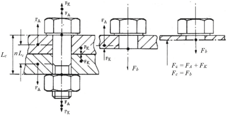
Figure description:
Key Entities
- Fastener Assembly: A bolt and nut clamping two plates.
- Clamped Plates: Cross-sections of the materials held together.
- Loading Planes: Horizontal lines within the clamped material representing where forces act.
Dimensions and Parameters
- : Total clamped length of the joint.
- : The distance between the internal loading planes.
Forces
- : External axial load.
- : Clamping force (preload.
- : Total force in the bolt/fastener.
- : Resultant compressive force.
Equations
Figure 7-17 - Tension Joint Loading Planes and the Forces Acting within the Joint
Between the loading planes the joint’s internal compressive stresses are relieved by the effect of the external load, FA . Outside the loading planes the clamped material is subjected to extra compression effect of FA in addition to the clamping load, FK .
The effect of the loading plane factor on the joint diagram is shown in Figure 7-18. As n reduces, the effective fastener stiffness reduces and the effective joint stiffness increases (see Reference 7.4). Hence, the closer the loading planes, the smaller the fastener load increment and the larger the preload relief in the clamped parts.
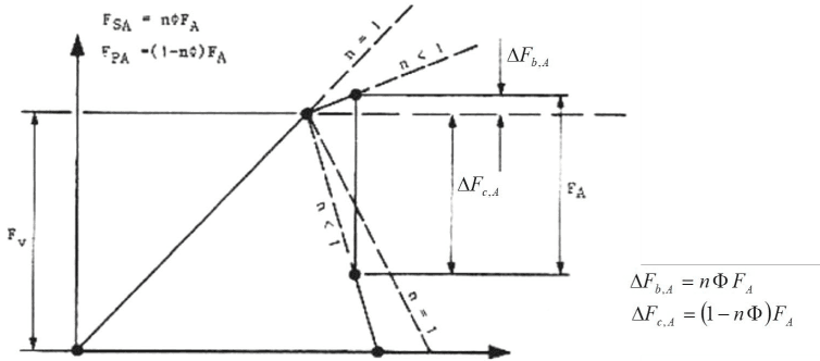
Figure description:
Schematic Representation of Force Components
Force Component Schematic for n=1 and n<1 Cases
Legend
- n = 1 — color: black; symbol: Dashed lines
- n < 1 — color: black; symbol: Solid and dashed lines
Annotations
- n = 1 (text_label - position: associated with dashed line branches)
- n < 1 (text_label - position: associated with solid/dashed line branches)
- F_v (text_label - position: vertical axis dimension)
- F_A (text_label - position: vertical dimension on right)
- Delta F_b,A (text_label - position: upper vertical increment on right)
- Delta F_c,A (text_label - position: lower vertical increment on right)
| Element | Label / Formula | Description |
|---|---|---|
| Equation (Top Left) | First component force equation | |
| Equation (Top Left) | ) | Second component force equation |
| Equation (Bottom Right) | Upper force increment relative to baseline | |
| Equation (Bottom Right) | ) | Lower force increment relative to baseline |
| Vertical Axis Height | Baseline force level | |
| Total Vertical Span | Combined force range () | |
| State Parameter | Baseline case represented by dashed lines | |
| State Parameter | Deviated case represented by solid and dashed lines |
Notes: The figure illustrates the geometric and algebraic relationships between various force components (), , , and parameters , , and . It shows how force increments sum up to the total span .
Figure 7-18 - Joint Diagram for Loading Planes within the Joint (n < 1)
7.7.1.2 Approximate Method
The loading plane factor depends on the deformation of the joint caused by the preload. For uncritical verification purposes with simple joint geometries the loading plane factor can be set to 0,5, which assumes that the loading planes are at the centre of each flange.
7.7.1.3 Experimental Method
A more precise value for the loading plane factor can be determined from testing by use of the relation,
where; δ is the effective compliance of the joint (equal to the relative deflection of the loading planes j for 1N of externally applied axial load), and 2 are the deflections of the points of action of the external load, and fuh,1 and fuh,2 are the deflections of the under-head and under-nut bearing surfaces under the same external load.
Equation [7.7.1] cannot be applied without knowing of the axial deflections of the under-head and under-nut bearing surfaces and the loading planes due to the externally applied axial load. These deflections can be determined by test or FEM modelling.
7.7.1.4 Geometric Analysis Method
The deformation of the joint is depends strongly on its geometry. For a concentric axially loaded joint, the determination of the loading plane factor is relatively simple provided there is continuous and uniform contact pressure between the flanges. In such cases, the loading plane factor depends only on the following parameters:
- Duh,brg The under-head bearing diameter (or diameter of the washer if it is assumed to be stiff)
- Dh The hole diameter
- ak The distance between the edge of the bearing surface under the fastener head and the point load introduction of the external force
- ar The shortest distance between the edge of the bearing surface and the edge of the clamped parts
- hk The distance between the point of load introduction and the interstice
These geometric parameters are defined in Figure 7-19.
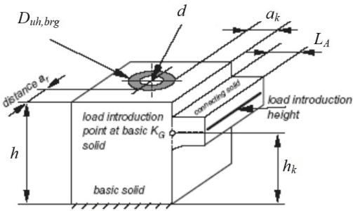
Figure description:
The image illustrates the geometric parameters for determining a loading plane factor.
Key Entities and Labels:
- Basic solid: The primary block structure.
- Connecting solid: A smaller block attached to the side of the basic solid.
- Load introduction point at basic solid: Indicated by a point where the connecting solid meets the basic solid.
- Load introduction height: Indicated by a horizontal line on the connecting solid.
- : Diameter of the bearing surface area on top of the basic solid.
- : Inner diameter of the hole/opening.
- : Total height of the basic solid.
- : Height from the base to the center of the connecting solid.
- : Width of the connecting solid.
- : Distance from the basic solid to the load introduction height line.
- distance : Horizontal distance from the edge of the basic solid to the center of the hole.
Figure 7-19 - Geometry for Determination of Loading Plane Factor
Using the geometric analysis method, the joint is first extracted from its environment by making a cut at a position where the inner moment is zero (see Figure 7-20). In joints with multiple fasteners there are interference effects between neighbouring fasteners, causing the clamped parts to be stiffer than in case of a single fastener joint. This effect is due to the mutual obstruction of lateral deformations by the neighbouring fasteners. This problem can be solved by using the distance between the hole edges of two neighbouring holes as the region of the deformation cone for the calculation of the clamped parts compliance, δ . c
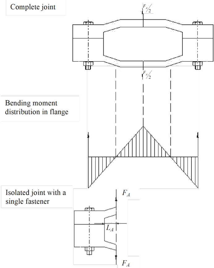
Figure description:
Mechanical Joint and Flange Bending Analysis
Bending moment distribution in flange
Annotations
- Complete joint (text_label - position: Top section of the figure)
- Bending moment distribution in flange (text_label - position: Middle section of the figure)
- Isolated joint with a single fastener (text_label - position: Bottom section of the figure)
- F_A / 2 (text_label - position: Applied load at the center of the complete joint assembly)
- F_A (text_label - position: Applied load at the centerline of the isolated joint model)
- L_A (text_label - position: Distance from the fastener centerline to the joint centerline in the isolated model)
- Vertical dashed lines (vertical_line - position: Indicates alignment of fastener axes and joint centerline across all diagrams)
| Position | Bending Moment (Qualitative) |
|---|---|
| Left Fastener Centerline | Negative Peak |
| Zero-crossing (Left) | 0 |
| Joint Centerline | Positive Peak |
| Zero-crossing (Right) | 0 |
| Right Fastener Centerline | Negative Peak |
Notes: The figure illustrates the mechanical analysis of a bolted flange joint. It shows the assembly ('Complete joint', its corresponding 'Bending moment distribution in flange', and an 'Isolated joint with a single fastener' model. The bending moment graph depicts a positive peak at the joint's centerline and negative peaks at the fastener axes, which are spaced by a distance L_A from the center.)
Figure 7-20 – Extraction of the Joint from its Environment
After extracting the joint from its environment, it be split into a ‘basic body’ and a ‘connector body’. The basic body determines the elastic properties of the joint, including the deformation cone. The connector body is the part of the joint where the external forces are applied. The point of external force introduction into the basic body KG is assumed to be at the horizontal mid-plane of the connector body.
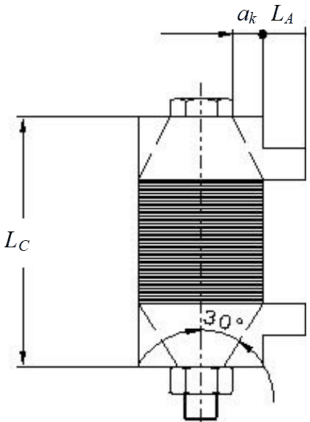
Figure description:
The image depicts a schematic diagram of a bolted joint assembly.
Key Entities and Dimensions:
- Bolt and Nut: A vertical bolt assembly with a hexagonal head at the top and a nut at the bottom.
- : Dimension indicating the total clamped length of the joint.
- : Lateral distance from the bolt centerline to the edge of the upper clamped component.
- : Distance from the bolt centerline to an external loading point.
- 30° Angle: Indicates a cone of influence originating from the nut and bolt head contact surfaces.
- Shaded/Hatched Zone: A central region between the upper and lower conical sections representing the compressed area of the joint.
- Centerline: A dashed vertical line passing through the center of the bolt.
Figure 7-21 - The Basic and Connector Bodies
7.7.2 Simple Calculation of the Loading Plane Factor
7.7.2.1 Overview
This Section presents a simple method for determining the loading plane factor. The method is based on a 2-dimenional representation of the joint and it makes the following assumptions:
- • No external moments act on the fastener (but the moment acting on the fastener due to the external force is considered)
- • The joint’s flanges have no gapping
- • All clamped parts in the joint have the same modulus of elasticity
- • The joint body is of prismatic shape.
- • The product of the parameters concerning the 3-dimensional nature of the joint can be conservatively estimated by kas * kdh *kdw = 0,8 (see Section 7.7.3.3 for the analytical definition of these parameters).
7.7.2.2 Joint Types for the Simple Method
Most commonly used joints can be approximated by a class of simplified joints shown in Figure 7-22 according to the point of force introduction into the joint. It is important that the interstice lies inside the shaded zone of the corresponding diagram. This zone defines the region where evenly distributed compression is assumed, and is assumed to have a cone half angle of 30°.
Figure 7-22 shows only nut-tightened joints, however the joint types 1, 2 and 4 are also applicable to threaded hole joints. In these cases the lower flange acts as the insert and the dimension Lc is only the thickness of the upper flange.
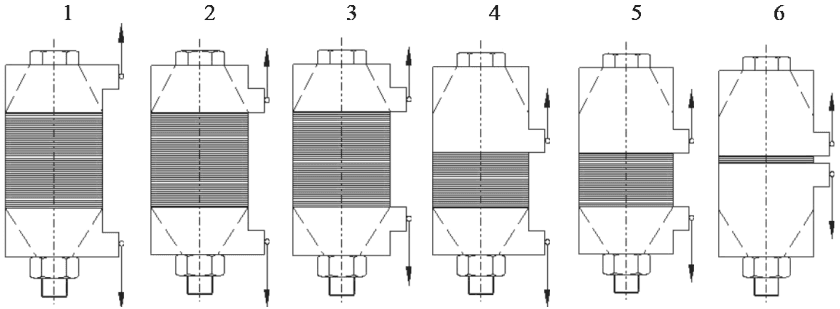
Figure description:
The image displays six diagrams, labeled 1 through 6, each depicting a bolted joint assembly.
Key entities and features:
- Bolted Joint Assemblies: Each diagram shows a central vertical bolt with a hexagonal head at the top and a nut at the bottom, securing multiple horizontal plates.
- Force Introduction Points: Small circles on the right side of the assemblies indicate where force is applied.
- Directional Force Vectors: Arrows pointing away from the force introduction points indicate the direction of the applied load.
- Variations (1-6: The diagrams show different configurations for the number of plates, the thickness of the clamped parts, and the specific locations where the tensile forces are applied relative to the bolt and joint interface.
Figure 7-22 – Joint Types According to the Points of Force Introduction
7.7.2.3 Interpolation Table for the Simple Method
The loading plane factor is read from Table 7-2. For intermediate parameter values linear interpolation is applicable.
| LA / LC | ak / LC | JOINT TYPE (FROM FIGURE 7-22) | |||||
|---|---|---|---|---|---|---|---|
| 1 | 2 | 3 | 4 | 5 | 6 | ||
| 0,0 | 0,0 | 0,70 | 0,57 | 0,44 | 0,42 | 0,3 | 0,15 |
| 0,1 | 0,55 | 0,46 | 0,37 | 0,34 | 0,25 | 0,14 | |
| 0,3 | 0,30 | 0,30 | 0,26 | 0,25 | 0,22 | 0,14 | |
| ≥0,5 | 0,13 | 0,13 | 0,12 | 0,12 | 0,10 | 0,07 | |
| 0,1 | 0,0 | 0,52 | 0,44 | 0,35 | 0,33 | 0,24 | 0,13 |
| 0,1 | 0,41 | 0,36 | 0,30 | 0,27 | 0,21 | 0,12 | |
| 0,3 | 0,22 | 0,21 | 0,20 | 0,16 | 0,15 | 0,10 | |
| ≥0,5 | 0,10 | 0,10 | 0,09 | 0,08 | 0,07 | 0,06 | |
| 0,2 | 0,0 | 0,34 | 0,30 | 0,26 | 0,23 | 0,19 | 0,11 |
| 0,1 | 0,28 | 0,25 | 0,23 | 0,19 | 0,17 | 0,11 | |
| 0,3 | 0,16 | 0,16 | 0,15 | 0,12 | 0,12 | 0,09 | |
| ≥0,5 | 0,07 | 0,07 | 0,07 | 0,06 | 0,06 | 0,06 | |
| ≥0,3 | 0,0 | 0,16 | 0,16 | 0,16 | 0,14 | 0,14 | 0,10 |
| 0,1 | 0,14 | 0,14 | 0,14 | 0,13 | 0,13 | 0,10 | |
| 0,3 | 0,12 | 0,12 | 0,12 | 0,10 | 0,10 | 0,08 | |
| ≥0,5 | 0,04 | 0,04 | 0,04 | 0,03 | 0,03 | 0,03 | |
7.7.3 Analytical Calculation of the Loading Plane Factor
7.7.3.1 Overview
The loading plane factor can be determined analytically by the method presented in this section, although it is normally considered too complex for hand calculations. Thus, it is expected that the method presented here is mainly used in computer programs (or spreadsheets, etc.) for fastener analysis.
It is assumed that height of the connector body is relatively small compared to the thickness of the flanges and thus, the load introduction can be represented by a point force. Also, it is assume that the joint consists of two flanges (such as shown in Figure 7-23), each of which can be treated separately.
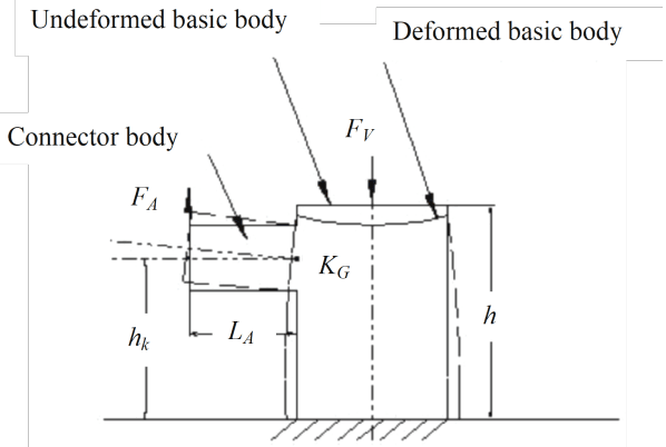
Figure description:
- Entities:
- Undeformed basic body: Represented by solid outlines of the main vertical structure.
- Deformed basic body: Represented by dashed outlines showing the vertical structure bowing outward and the top surface curving inward.
- Connector body: A horizontal projection on the left side of the basic body.
- Forces:
- : Vertical downward force applied to the center of the top surface.
- : Vertical upward force applied to the end of the connector body.
- Geometric Dimensions:
- : Total height of the basic body.
- : Height from the base to the centerline of the connector body.
- : Length of the connector body measured from the edge of the basic body.
- Parameters:
- : Point indicated at the interface between the connector body and the basic body.
The (overall) loading plane factor of the joint is based on loading plane factors for the two flanges according to,
where; and are the loading plane factors for the upper and lower flanges respectively, and and are the compliances of the upper and lower flanges respectively.
7.7.3.2 Loading Plane Factor for a Single Flange
The loading plane factor for a single flange is given by,
[7.7.3] (only valid for )
where and are the general loading plane and moment conduction factors respectively, which are given in the following Sections.
7.7.3.3 The Moment Conduction Factor
The moment conduction factor, , accounts for the influence of the position of the connector body relative to the compression cone and the parameter , and is calculated by,
where;
- nG is the loading plane factor of the basic body (see 7.7.3.4),
nG* is the loading plane factor of the basic body whose parameter ak/h is reduced by 0,1, and;
is the ratio of the 2D loading plane factors, where is calculated with a ratio that is reduced by 0,1, and is moved into the region of evenly distributed compression (for the calculation of both factors)
Figure 7-24 shows the principal trends of over the height of a flange.
Equations [7.7.3] and [7.7.4] show that the loading plane factor is reduced if the connector body lies in the spreading zone of the compression cone. In some cases this leads to negative values for , which can be interpreted as a one-sided gapping of the joint due to the bending effect of the applied load.
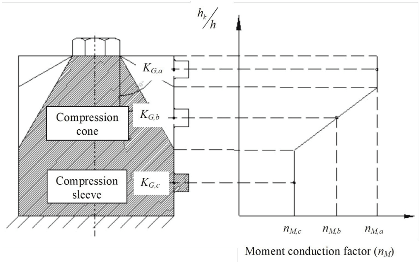
Figure description:
Moment Conduction Factor Distribution
Relation between Moment Conduction Factor and Dimensionless Height
Annotations
- Compression cone (text_label - position: upper shaded region of diagram)
- Compression sleeve (text_label - position: lower shaded region of diagram)
- 30° (text_label - position: half-angle of the compression cone)
- K_{G,a} (text_label - position: height level a, corresponding to n_{M,a} on the curve)
- K_{G,b} (text_label - position: height level b, corresponding to n_{M,b} on the curve)
- K_{G,c} (text_label - position: height level c, corresponding to n_{M,c} on the vertical section)
| Moment conduction factor (n_M) | h_k / h |\n| :--- | :--- |\n| n_{M,c} | 0 |\n| n_{M,c} | level of K_{G,c} |\n| n_{M,c} | level of sleeve-cone boundary |\n| n_{M,b} | level of K_{G,b} |\n| n_{M,a} | level of K_{G,a} |
Notes: The diagram illustrates how the moment conduction factor n_M varies with the height ratio h_k/h for different sections of a bolted joint assembly. The factor is constant (n_{M,c} within the compression sleeve section and increases linearly through the compression cone section up to n_{M,a}.)
Figure 7-24- Moment Conduction Factor Variation with the Connector Body Position7.7.3.4 The General Loading Plane Factor
The general loading plane factor of the joint is calculated by,
where and is the loading plane factor of an equivalent two-dimensional joint calculated by,
where the geometric variables , , and are defined in Figure 7-19, and the factors , & account for the influence of the 3D spatial extension of the joint and are given by,
Equations [7.7.5] to [7.7.8] are valid in the ranges,