A simple example showing the effects of dynamic loading is given in Figure 7-28. Here, an alternating external axial load varying from zero to FA is applied to a joint. The fastener experiences a dynamic load with amplitude of ∆ A /2.
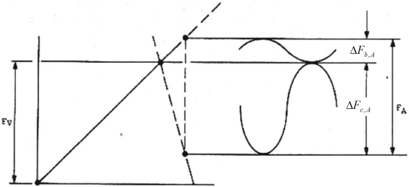
Figure description:
Force-Deformation Diagram of a Bolted Joint under External Load (Rötscher's Diagram - Extraction of Parameters and Relationships. Additional notes: The diagram represents the classic joint diagram used in mechanical engineering to determine how an external load is shared between the bolt and the clamped members. The intersection point of the two diagonal lines represents the assembly state with preload F_V. Upon application of an external force F_A, the bolt stretches further (increasing its force by delta_F_b,A while the clamped parts decompress (decreasing their clamping force by delta_F_c,A.
Joint Diagram (Preload Diagram for a Bolted Joint
Legend
- Bolt stiffness characteristic — color: black; symbol: Solid diagonal line with a positive slope starting from the origin.
- Clamped parts stiffness characteristic — color: black; symbol: Solid diagonal line with a negative slope intersecting the bolt line at (x, F_V.
- Dynamic load component — color: black; symbol: Sine-wave shapes representing alternating force components around the static load levels.
Annotations
- F_V (text_label - position: Intersection height of the bolt and part stiffness lines on the vertical axis.)
- F_A (text_label - position: The total vertical distance between the extended bolt stiffness line and the part stiffness line at the loaded state.)
- delta_F_b,A (text_label - position: The vertical distance from the preload line (F_V up to the bolt stiffness line.))
- delta_F_c,A (text_label - position: The vertical distance from the preload line (F_V down to the clamped parts stiffness line.))
| Parameter | Symbol | Relation / Definition |
|---|---|---|
| Preload Force | F_V | The initial clamping force applied to the joint at assembly. |
| External Axial Load | F_A | The total additional axial force applied to the joint. |
| Additional Bolt Force | delta_F_b,A | The part of the external load F_A that is carried by the bolt. |
| Clamping Force Reduction | delta_F_c,A | The part of the external load F_A that reduces the compression in the clamped parts. |
| Equilibrium Relationship | F_A | F_A = delta_F_b,A + delta_F_c,A |
Figure 7-28 – Joint Diagram Showing a Dynamic External Load
The dynamic stress amplitude in the fastener due to the external load is given by,
where is the fastener stress area (see Section 5.4).
Figure 7-29 is a typical S-N curve that relates the applied stress in a component to its number of cycles to failure. As reduces, the number of cycles to failure increases, until the stress is below a certain threshold , after which the fastener is termed fatigue resistant.
In Section 7.4 it was shown that ∆ A is reduced by decreasing the fastener’s stiffness relative to that of the clamped parts. Hence, to improve fatigue resistance, it is recommended to use reduced shank fasteners.
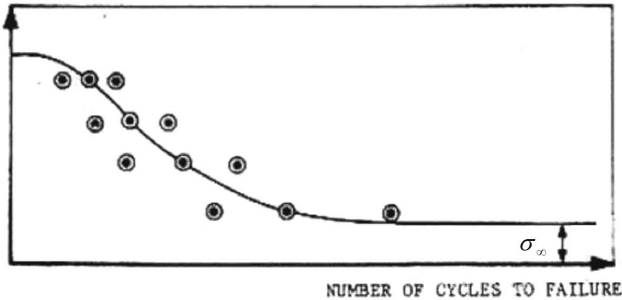
Figure description:
Number of Cycles to Failure vs Stress
Fatigue (S-N Curve
Annotations
- σ∞ (text_label - position: y = 0.45)
| Number of Cycles to Failure (relative) | Stress (relative) | Series |
|---|---|---|
| 0.00 | 0.89 | Fitted Curve |
| 0.09 | 0.79 | Data Points |
| 0.10 | 0.85 | Fitted Curve |
| 0.14 | 0.79 | Data Points |
| 0.14 | 0.64 | Data Points |
| 0.19 | 0.79 | Data Points |
| 0.20 | 0.76 | Fitted Curve |
| 0.21 | 0.70 | Data Points |
| 0.21 | 0.54 | Data Points |
| 0.27 | 0.70 | Data Points |
| 0.29 | 0.59 | Data Points |
| 0.30 | 0.63 | Fitted Curve |
| 0.34 | 0.45 | Data Points |
| 0.40 | 0.59 | Data Points |
| 0.40 | 0.53 | Fitted Curve |
| 0.48 | 0.45 | Data Points |
| 0.50 | 0.47 | Fitted Curve |
| 0.60 | 0.45 | Fitted Curve |
| 0.64 | 0.45 | Data Points |
| 1.00 | 0.45 | Fitted Curve |
Notes: The chart illustrates the relationship between cycle counts and failure stress, identifying the fatigue limit σ∞. Data points represent individual experimental results, and the solid line represents a fitted fatigue curve. Since no numerical scale is provided on the axes, values are estimated on a relative scale from 0 to 1.
Figure 7-29 – Typical S-N Curve (For a Given Mean Stress)