ANALYSIS CRITERIA
A.1 Purpose of Appendix A
This Appendix provides an explanation and justification of fastener analysis criteria.
A.2 Accounting for Preload Variation when Installing Fasteners with Torque Control (Supplement to Section 4.3.1)
This section is intended to clarify the criteria in section 4.3.1 and to provide additional guidance regarding calculation of maximum and minimum preloads when using torque control.
The relationship between preload and torque can be characterized by a statistical distribution. Multiple tests have shown that this distribution is usually normal (Gaussian), and the mean and standard deviation can be inferred from the test data with varying degrees of confidence. Thus, for a given input torque, there is a normal probability distribution for the resulting preload having a mean and a standard deviation.
The relationship between the nominal (mean) initial preload, Ppi-nom , and the nominal effective torque, T, can be expressed as
where 1/Knom is the nominal (mean) of the inverse of the nut factor (1/K) and D is the nominal bolt diameter.
Maximum initial preload is calculated by modifying Eq. 3 as
where is the preload variation, and Tmax is the maximum effective torque. For use in separation analysis of separation-critical joints, minimum initial preload is calculated by modifying Eq. 4 as
(Eq. 26a)
where Tmin is the minimum effective torque. For use in separation analysis of joints that are not separation-critical and joint-slip analysis, minimum initial preload is calculated by modifying Eq. 5 as
The maximum and minimum effective torques are calculated as follows:
- • If the installation torque is specified as some value or range “above running torque,” or if a locking feature that does not introduce a running torque is used,
where Ts-max and Ts-min are the maximum and minimum specified torques, respectively. For example, if the torque specification is “60 ± 3 in-lb above running torque,” Tmax = Ts-max = 63 in- lb and Tmin = Ts-min = 57 in-lb.
- • Otherwise, the maximum and minimum effective torques are calculated by subtracting the extreme values of running torque from the specified torques:
where Tbr-min is the minimum breakaway torque specified for the locking feature (can be conservatively set equal to zero) and TL-max is the maximum locking torque (running torque) specified for the locking feature.
Section 4.3.2 herein requires that calculation of the nominal initial preload, Ppi-nom , be substantiated by test. Because the torque-preload relationship is not truly linear, as Eq. 24 suggests, the most accurate method of determining Ppi-nom for a given effective torque, T, is to compute the sample mean (average) preload measured at that effective torque during the tests:
(Eq. 31)
where j is the test number, Ppi-j is the initial preload obtained in the j-th test, and m is the number of tests. The nominal nut factor is then calculated by rearranging Eq. 24:
Section 4.3.3 herein requires that, when using torque control and without applicable data showing otherwise, the preload variation, , for use in Eq. 25 and 26a and b (in all analyses except separation analysis of separation-critical joints) should be 25 percent for fasteners lubricated at assembly and 35 percent for non-lubricated and as-received fasteners. Historic NASA criteria have specified that when using torque control of preload, lubricated bolts have a preload uncertainty (variation), , of 25 percent from a typical (nominal or mean) value, and non-lubricated bolts have a preload uncertainty of 35 percent from a typical value. It historically has been assumed that these preload uncertainties envelop some large, but undefined, percentage of the probability distribution. Section 4.3.3 goes on to say, “When using the alternate (not the statistical) method for non-separation critical joints, if the test-measured variation exceeds the values stated above, then the test-measured variation should be used or methods for reducing the preload variation should be pursued.” The “actual extreme variation” referred to here is calculated from test data as two values, a-max and a-min:
or
where Ppi-maxa and Ppi-mina are the actual maximum and minimum initial preloads measured in the torque-preload tests. Eq. 33 applies to the establishment of when calculating maximum preload, and Eq. 34 applies when calculating minimum preload. When calculating maximum preload, is then the greater of a-max and the default value (0.25 lubricated, 0.35 non- lubricated). When calculating minimum preload, is then the greater of a-min and the default value (0.25 lubricated, 0.35 non-lubricated).
Per section 4.3.3, calculation of minimum initial preload for separation analysis of separation- critical joints requires to be derived from test data as the value determined to be at a statistical basis of 90 percent probability and 95 percent confidence (two-sided distribution). This value, 90/95, may also be used per section 4.3.3 to calculate maximum preload or to calculate minimum preload for joints that are not separation-critical. To determine the 90/95 value, first calculate the unbiased sample standard deviation, pi, from the collected sample of initial preloads for a given torque:
The preload variation at 90 percent probability and 95 percent confidence is then
where s is the number of standard deviations from the mean applicable to 90 percent probability and 95 percent confidence; s varies with sample size, m, as given in Table 5, Two-Sided 90/95 Tolerance Limit Factors for a Normal Distribution (Odeh and Owen, 1980).
| m | s | m | s | m | s | m | s |
|---|---|---|---|---|---|---|---|
| 2 | 31.092 | 12 | 2.670 | 22 | 2.272 | 40 | 2.055 |
| 3 | 8.306 | 13 | 2.601 | 23 | 2.251 | 45 | 2.024 |
| 4 | 5.368 | 14 | 2.542 | 24 | 2.232 | 50 | 1.999 |
| 5 | 4.291 | 15 | 2.492 | 25 | 2.215 | 55 | 1.978 |
| 6 7 | 3.733 3.390 | 16 17 | 2.449 2.410 | 26 27 | 2.199 2.184 | 60 65 | 1.960 1.944 |
| 8 | 3.156 | 18 | 2.376 | 28 | 2.170 | 70 | 1.931 |
| 9 | 2.986 | 19 | 2.346 | 29 | 2.157 | 80 | 1.908 |
| 10 | 2.856 | 20 | 2.319 | 30 | 2.145 | 90 | 1.890 |
| 11 | 2.754 | 21 | 2.294 | 35 | 2.094 | 100 | 1.875 |
As an example, consider a torque-preload test of 10 sets of fastening system hardware, with each cycled 3 times in the as-received condition. The effective torque, T, is 450 in-lb, and the nominal bolt diameter, D, is 0.375 in. The measured preloads are listed in Table 6, Sample Data from 30 Torque-Tension Tests (Actual Test Data).
| Bolt 1 | Bolt 2 | Bolt 3 | Bolt 4 | Bolt 5 | Bolt 6 | Bolt 7 | Bolt 8 | Bolt 9 | Bolt 10 | |
|---|---|---|---|---|---|---|---|---|---|---|
| Test 1 | 7760 | 4010 | 3587 | 4635 | 4920 | 3797 | 4462 | 4940 | 6220 | 4780 |
| Test 2 | 7229 | 4310 | 3900 | 4322 | 4475 | 3812 | 4132 | 4219 | 6100 | 4685 |
| Test 3 | 6080 | 4291 | 3054 | 4804 | 3910 | 3303 | 4090 | 4550 | 6062 | 5180 |
From Eqs. 31 through 36, with n = 30 and s = 2.145,
To calculate , (higher of and 0.35).
Alternatively, it is acceptable to use , calculated as follows:
To calculate , if the joint is not separation-critical, (higher of and 0.35), that is less penalizing than the alternative of using .
Note that, in the above example, there is unusually high variation in the initial preloads obtained for the given torque. In such a case, it is advisable to investigate the cause of such high variation in and take appropriate steps such as modifying the installation process by use of lubrication or selecting different fastening system hardware.
A.2.1 Rationale for Eqs. 5 and 26b
When performing slip analysis, the concern related to preload is not the variation in preload for a single fastener, it is the variation in total preload for the joint. Because the preload for any single bolt in the joint has a probability distribution for a given torque, then the total preload for the bolt pattern has a probability distribution. The total preload equals the mean preload for the bolts in the pattern multiplied by the number of fasteners, so the probability distribution for total preload is the same as the probability distribution for the mean preload for the bolts in the pattern. This distribution is referred to as the distribution of the means, and it is characterized using the Central Limit Theorem as having a mean equal to the mean of the population (the mean of the distribution for any single bolt) and a standard deviation equal to the standard deviation of the population divided by the square root of the number of bolts in the bolt pattern. So, for a joint containing a number of bolts, , the probability distribution for the total preload for the n-bolt pattern has a mean, , and a standard deviation, . It can be assumed that the distribution of the means is normal.
The Central Limit Theorem states that the distribution of the means approaches a normal distribution as the size of the sample used to calculate the mean approaches infinity, even if the distribution of the population is non-normal. For practical purposes, the distribution of the
means is near normal when the sample size is greater than or equal to 30 (Spiegel, 1961, p. 144). The distribution of the means “tends to be normally distributed even for relatively small n [sample size] as long as no single element or small group of elements has a dominating variance and the element distributions do not deviate extremely from a normal distribution” (Hahn and Shapiro, 1967, p. 73). The standard deviation of the distribution of the means is also known as the “standard error.”
When performing separation analysis, part of the concern is separation of the entire joint; and part of the concern is local separation near a single fastener. The minimum preload used for separation analysis of separation-critical joints must be derived by test at the statistical probability and confidence specified in section 4.3.1. For joints that are not separation-critical, it is acknowledged that the consequence of local separation in a joint with multiple fasteners is not as severe as the consequence of rupture or detrimental yielding; so it is acceptable to base the separation analysis on a minimum preload that is progressively less conservative as the number of fasteners in the pattern increases. Although the Central Limit Theorem does not apply to preload at a single fastener (it applies only to total preload for a bolt pattern and thus separation analysis for the overall joint), it is acceptable for separation analysis at the highest-loaded fastener in a non-separation-critical joint to use a minimum preload calculated the same way in which it is calculated for slip analysis, as noted above and specified in section 4.3.1.
Separation under cyclic applied load, whether for the entire joint or local to a fastener, is undesirable as it causes more fatigue damage in the fastener. Fatigue analysis, however, must account for the full range in preload with uncertainty as specified in section 4.3.1. When assessing non-separation-critical joints with multiple fasteners, if the pattern has a positive margin of safety for separation at the joint level but the highest-loaded fastener in the pattern has a negative margin of safety for separation at the local level, fatigue analysis must account for the increase in tension due to separation.
A.3 Short-Term Relaxation of Preload (Supplement to Section 4.3.1)
Table 1 provides an adjustment for short-term relaxation of preload. Such relaxation is a well- documented effect attributed to embedment that results from localized yielding at interfaces. When calculating minimum preload, it is acceptable in most cases to reduce the minimum initial preload by 5 percent for short-term relaxation. Higher losses of preload have been reported as a result of short-term relaxation due to stack up of washers, smaller-diameter washers, low-yield strength materials, etc. In such cases, even for all-metal threaded fastening systems, larger reductions may be necessary.
A.4 Use of a Load-Introduction and Stiffness Factor (Supplement to Sections 4.4.1 and 4.4.2)
The load-introduction factor (LIF), n, as used in Eq. 17 and Eq. 8, accounts for the effects on the tensile bolt load due to the joint geometry and location of the external load. The LIF can be derived based on a linear spring model as shown in “The Mechanism of Bolt Loading” (H. M. Lee, NASA TM-108337), or by including off-center tensile loads and flange bending effects as
shown in “Effect of Separating Load Eccentricity on the Clamp Load Loss in a Bolted Joint Using a Strain Hardening Model” (Nassar & Ganganala, ASME Journal of Pressure Vessel Technology, April 2011, Vol. 133). Verein Deutscher Ingenieure (VDI) 2230, Systematic Calculation of High Duty Bolted Joints, Joints with One Cylindrical Bolt, provides the LIF for various joint geometry characteristics based on analysis and experiment. The LIF, n, may be determined using the aforementioned references, and varies between 0 and 1 depending on the joint geometry and the point of application of the external load.
Historically, in National Space Transportation System (NSTS) 08307, Criteria for Preloaded Bolts, the LIF has been defined solely as a length ratio of the thickness of the relieved joint materials between loading-plane locations Llp , to the total thickness of the joint L, as
where L and Llp are as defined in Figure 3, Dimensions Used to Calculate the Geometric Load- Introduction Factor, for three types of joints. Because this definition of the LIF is characterized solely by intuitive geometric considerations, it is hereafter denoted as the geometric LIF.
The value for the LIF can be calculated using various methods such the methods of NSTS 08307, NASA TM-108337, or VDI 2230. The method found in NASA TM-108337 is denoted herein as the stiffness-based LIF, further explained below, and is considered more accurate than other handbook solutions since it accounts for more realistic stiffness considerations of the bolted joint. A method that provides even more accuracy, assuming the bolted joint design is properly represented, is finite element analysis.
The stiffness-based LIF usually allocates less external load to the bolt than does the geometric LIF. Therefore, if the stiffness-based LIF is used, care must be taken to make sure that accurate external loads (by considering load amplifying affects such as prying action and material nonlinearities, etc.) are used so that non-conservative margins of safety are avoided.
This idealization of the preloaded bolted joint assumes that the tensile component of the external load acts collinearly with the bolt axis (and ignores the effect of dimension b, as shown in Figure 3). This idealization also assumes that this load and its reaction acts as uniform pressures on loading-planes perpendicular to the bolt axis, separated by a distance equal to the thickness of the relieved joint material, Llp , and being bounded by the joint compression zone boundaries. It can be shown analytically that this LIF is based on the implicit assumption that the compression zone is of constant area and of uniform modulus of elasticity. Both of these implicit assumptions are generally not true, in that the compression zone usually has some type of varying geometry, and clamped members also commonly consist of different materials.
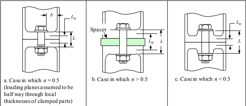
Figure description:
Key Entities and Information:
- Subject: Dimensions used to calculate the geometric load-introduction factor for bolted joints.
- Case a (n = 0.5: Loading planes are assumed to be halfway through the local thicknesses of clamped parts.
- Case b (n > 0.5: Includes a green-shaded "Spacer" element between clamped parts.
- Case c (n < 0.5: Variation in loading plane relative to thickness.
- Labeled Dimensions:
- b: Distance from bolt centerline to the edge of the clamped member.
- L: Total thickness of the clamped assembly between the bolt head and nut.
- L_lp: Distance between the designated loading planes.
- Components: Hex bolts, washers, nuts, and clamped members with internal recesses.
Figure 3—Dimensions Used to Calculate the Geometric Load-Introduction Factor
A.4.1 Derivation of the Stiffness-Based Load-Introduction Factor
A more detailed derivation of the load-introduction and stiffness factors is provided in NASA TM-108377 and is summarized here. Consider a preloaded bolted joint idealized by the following system of springs (represented as stiffness values), as shown in Figure 4, Preloaded Joint Represented by Springs, where kb is the bolt stiffness, kc is the joint stiffness, and Pt is the external tensile load. The joint is idealized into 4 regions, each region being demarcated by one of the following features: point 3 being a reference plane; points 2 and 4 at which the external tensile load acts on the joint; point 1 being the interface between the bolt head and clamped members; and point 5 being the interface between the nut (or insert) and clamped members. These four regions, in the most general case, will exhibit different stiffness values (due to varying modulus of elasticity of the individual clamped members within the region, and portion of frustum compression zone contained within the region), and this is represented by the product of the joint stiffness kc and a variable A, B, C, and D, as shown in Figure 4.
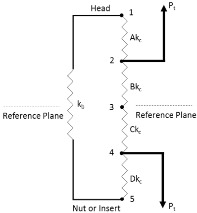
Figure description:
Diagram: Preloaded Joint Represented by Springs
- Entities:
- Head: Located at the top, connected to point 1.
- Nut or Insert: Located at the bottom, connected to point 5.
- Reference Plane: Indicated by a horizontal dashed line passing through point 3 and the middle of spring .
- External Load (: Represented by two bold arrows pointing in opposite directions, originating from point 2 (upward and point 4 (downward.
- Stiffness Elements (Springs:
- : Represents the bolt, connected between the "Head" and "Nut or Insert" structures.
- : Connected between points 1 and 2.
- : Connected between points 2 and 3.
- : Connected between points 3 and 4.
- : Connected between points 4 and 5.
- Numbered Points: Points 1, 2, 3, 4, and 5 form a vertical series of nodes for the spring segments.
Figure 4—Preloaded Joint Represented by Springs
The four regions should not be confused with the number of clamped members in any given joint. Any number of clamped members, indicated by springs (stiffness values), can be represented by the four regions as shown in Figure 4 using the relationships between spring stiffness in series and the known joint stiffness. For example, writing the stiffness for the region between points 1 and 2 yields Eq. 38. Similar equations can be written for the other regions. The configuration shown in Figure 4 covers any number of clamped members.
Consider the clamped members from Figure 4 that are relieved upon application of the external load Pt . These clamped members are represented by stiffness values Bkc and Ckc . Because the joint is preloaded, these springs act in series. The combined stiffness is denoted as K2-3,3-4 and can be determined as
Consider the remainder of the system of Figure 4 consisting of the clamped members that are compressed upon application of the external load, represented by the stiffness values Akc and Dkc , and the bolt represented by the stiffness kb . Because the joint is preloaded, the springs act in series, and the combined stiffness is
The joint idealization shown in Figure 4 can be further simplified using the two stiffness values K2-3,3-4 and K1-2,4-5 as shown in Figure 5, Preloaded Joint Represented by Two Springs in Parallel, where K2-3,3-4 represents the combined stiffness of the clamped members that are relieved by application of an external tensile load, and K1-2,4-5 represents the combined stiffness of the clamped members that are compressed by the application of the external tensile load, in addition to the bolt member. The springs shown in Figure 5 act in parallel.
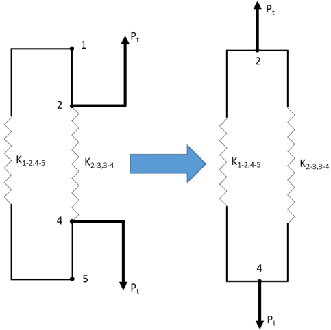
Figure description:
The image depicts two simplified mechanical spring models of a preloaded joint.
Left Diagram:
- Stiffness elements: Two parallel spring paths labeled and .
- Nodes: Labeled points 1, 2, 4, and 5.
- Applied Loads: External tensile forces ( applied at node 2 (upward and node 4 (downward.
Right Diagram (Simplified Model:
- Transformation: Indicated by a large blue arrow pointing from left to right.
- Stiffness elements: The same parallel spring paths, and , now shown in a simplified parallel configuration.
- Nodes: Labeled points 2 (top and 4 (bottom.
- Applied Loads: External tensile forces ( applied directly to nodes 2 and 4 in opposing directions.
Figure 5—Preloaded Joint Represented by Two Springs in Parallel
The effective stiffness of this entire system shown in Figure 5 can be represented by one stiffness denoted as Keff and written as
The relative displacement of points 2 and 4 with respect to each other can be written in terms of the external load as
Likewise, the relative displacement of points 2 and 4 with respect to each other can be expressed in terms of the amount of load reacted by the bolt excluding preload, or
Equating Eq. 44 and 45 yields
(Eq. 46)
that can be expressed as
where
and
The LIF represented in Eq. 48 is denoted herein as the stiffness-based LIF and is expressed in terms of the stiffness coefficients of the clamped members being relieved. This LIF may also be expressed in terms of the stiffness coefficients of the clamped members being compressed. Consider the stiffness of the entirety of clamped members. We have, therefore,
that leads to
Substituting Eq. 48 into Eq. 51 yields
The stiffness-based LIF can be expressed by either the stiffness coefficients of the clamped members being relieved by the external tension load, or the stiffness coefficients of the clamped members being further compressed by the external joint tensile load.
A.4.2 Limitation of the Geometry-Based Load-Introduction Factor
Consider the flexibility of the clamped members being relieved, as expressed in Eq. 39. Substituting Eq. 48 into Eq. 39 yields
The flexibility of the clamped members being relieved may be expressed in terms of a compression zone of arbitrary shape, A(x), and arbitrary modulus distribution, E(x), where x is the axial coordinate of the joint (i.e., along the length of the fastener), or
Likewise, for the entire length of the clamped members, one has
Substituting Eq. 54 and Eq. 55 into Eq. 53 yields
Eq. 56 is a general equation for the stiffness-based LIF. It is assumed that the axial component of the external load and its axial reaction act concentric to the bolt. The axial joint load and its axial reaction load are assumed to be applied uniformly on two parallel cross sections of the compression zone. These compression zone cross sections are assumed to be perpendicular to the bolt axis and separated by a distance equal to the thickness of the clamped members being relieved. The material is assumed to be linear elastic, and Poisson’s effects are ignored.
The geometric LIF, denoted herein as nG , is defined in NSTS 08307 and this NASA Technical Standard as the ratio of the thickness of the joint between force application points and the total thickness of the joint. This may be expressed using the variables of this work as
and depicted in Figure 6, Geometric Load-Introduction Factor.
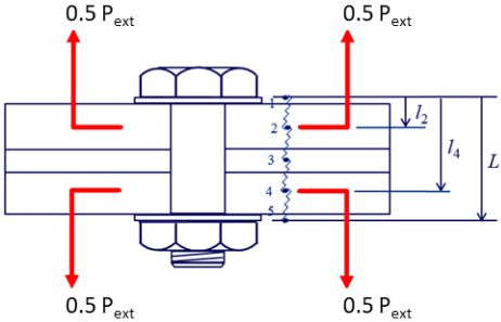
Figure description:
- Components: A bolted joint assembly consisting of a bolt, a nut, washers, and three clamped horizontal plates.
- Forces: Four external force vectors labeled are applied to the plates; two point upward from the top plate and two point downward from the bottom plate.
- Geometric Dimensions:
- : Total height of the clamped plates.
- : Distance from the top surface to the upper internal load application plane.
- : Distance from the top surface to the lower internal load application plane.
- Key Points: A vertical wavy line identifies five specific points/nodes numbered 1 through 5, corresponding to the surfaces and internal load planes.
By equating Eq. 56 and Eq. 57, we can express the geometric LIF in terms of the compression zone geometry and modulus distribution, or
Using the identity
it can be observed that the only way for Eq. 58 to be satisfied is that E and A not be functions of x, or E(x)A(x) is the constant EA. Therefore, the geometric LIF assumes that the compression zone is limited to a cross-section shape of constant area and of a single value for the modulus of elasticity throughout the length of the joint. In practice, this would be a cylindrical compression zone made of a single material. This conclusion is also supported in VDI 2230. The geometric LIF is inconsistent with the assumptions of a frustum-type compression zone geometry and with clamped members made of materials having different modulus of elasticity.
A.4.3 An Alternative to the Explicit Load-Introduction Factor
The geometric LIF nG , as defined in NSTS 08307 and in Eq. 37, has been used successfully for many years at NASA to predict the amount of external load allocated to the bolt through the product nG ϕ, per Eq. 8. For the bolted joint of Figure 3 (or shown as Figure 10 later in greater detail), the use of the stiffness-based LIF, n, allocates less load to the bolt than the use of the geometric LIF, nG . Finite element analysis (FEA) may be used to predict the product nϕ, and for
the joint in Figure 3 (or Figure 10), this product is closer to the value calculated using the stiffness-based LIF n, than is calculated using the geometric LIF nG . If it is assumed that FEA provides a reasonable approximation of the bolted joint behavior, it follows that the geometric LIF, nG, allocates too much load to the bolt for this particular joint.
With the continued development of FEA software, obtaining preloaded bolted joint characteristics, including prying effects due to off-axis bolt loading, by explicitly modelling a single bolted joint, has become computationally inexpensive. While it is beyond the scope of this NASA Technical Standard to provide FEA modelling guidance (model fidelity, mesh density, choice of elements, boundary conditions, and material properties), the FEA methodology to determine n , consists of the following steps:
- Explicitly model the clamped members, bolt, nut, and washers to the appropriate level of detail.
- Use the appropriate linear or nonlinear material properties.
- Apply a preload to the bolt.
- For the current preload, apply a range of external loads to the joint.
- Plot the load reacted by the bolt versus the external tension load component as shown in Figure 7, Predicting the Product n from Finite Element Analysis.
- Calculate the product n , as shown in Figure 7 that is the slope of the line in step 5.
- Go to step 3 and repeat for another preload level until the range of preloads are adequately covered.
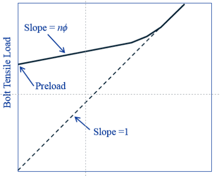
Figure description:
Bolt Tensile Load Diagram Relationship between bolt tensile load and external applied load showing preload and slope changes
Bolt Tensile Load vs. Applied Load
Annotations
- Slope = nϕ (text_label - position: Pointing to the initial linear segment of the solid line)
- Preload (text_label - position: Pointing to the y-intercept of the solid line at zero applied load)
- Slope = 1 (text_label - position: Pointing to the dashed reference line starting from the origin)
| Applied Load (Arbitrary) | Bolt Tensile Load (Solid Line) | Reference Line (Dashed Line, Slope = 1) |
|---|---|---|
| 0 | Preload | 0 |
| Low Load | Preload + (nϕ * Load) | Load |
| Transition Point | Transition Curve | Load |
| High Load | Load + Constant (Slope = 1) | Load |
Notes: The graph qualitatively shows how the tensile load in a bolt increases as external load is applied. It starts at an initial Preload value. The initial slope of the bolt load curve is nϕ (representing the joint's stiffness constant, which is significantly less than 1. As the external load increases, the curve transitions until its slope becomes 1, typically indicating joint separation where the bolt carries all additional applied load.)
Applied Tensile Load
Figure 7—Predicting the Product n from Finite Element Analysis
A.5 Bolt Analysis: Separation before Rupture (Supplement to Section 4.4.5)
Whether separation would occur before rupture can be determined based on test, analysis, or the logic flow in Figure 8, Determining Whether a Joint Separates before Rupture When Loaded Solely in Tension. If analysis is used, it should be based on the assumption of maximum preload.
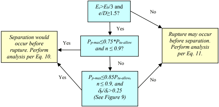
Figure description:
Flowchart: Determining Joint Separation vs. Rupture
Decision Points:
- Step 1: and ?
- No: Proceed to "Rupture may occur before separation. Perform analysis per Eq. 11."
- Yes: Proceed to Step 2.
- Step 2: and ?
- Yes: Proceed to "Separation would occur before rupture. Perform analysis per Eq. 10."
- No: Proceed to Step 3.
- Step 3: , , and (See Figure 9?
- Yes: Proceed to "Separation would occur before rupture. Perform analysis per Eq. 10."
- No: Proceed to "Rupture may occur before separation. Perform analysis per Eq. 11."
Key Entities/Variables:
- : Elastic moduli
- : Edge distance and diameter
- : Maximum preload
- : Allowable ultimate tensile load
- : Fitting factor/variable
- : Plastic and elastic deformation
- Eq. 10: Analysis for separation before rupture
- Eq. 11: Analysis for rupture before separation
Figure 8—Determining Whether a Joint Separates before Rupture When Loaded Solely in Tension
In Figure 8, Ec is the lowest elastic modulus of clamped parts excluding washers, Eb is the elastic modulus of the bolt material, e is the minimum edge distance (measured from center of hole to closest edge of any clamped part other than washers), p is the plastic deformation of the fastening system at rupture, and e is the elastic deformation of the fastening system at rupture. (See Figure 9, How to Quantify Ductility of a Fastening System from a Tension Test.)
Figure 9 shows a typical load-deflection curve for a bolt tested to failure in tension. The ratio of e to p depends on the fastener and the mating internally threaded part. To determine e and p, the bolt should be tested with an internally threaded part that is of the same specification as is used in the flight assembly in case the hardware combination leads to thread stripping as the mode of failure.
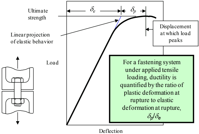
Figure description:
Ductility of a Fastening System
Load vs. Deflection Curve
Legend
- Actual Load-Deflection Curve — color: black; symbol: thick solid line
- Linear projection of elastic behavior — color: blue; symbol: thin solid line
Annotations
- Ultimate strength (horizontal_line - position: Load = 100)
- Linear projection of elastic behavior (line - position: y = 1.43x)
- Displacement at which load peaks (vertical_line - position: Deflection = 100)
- delta_e (dimension - position: Deflection from 0 to 70)
- delta_p (dimension - position: Deflection from 70 to 100)
- For a fastening system under applied tensile loading, ductility is quantified by the ratio of plastic deformation at rupture to elastic deformation at rupture, delta_p/delta_e (text_label - position: bottom right box)
| Deflection | Load (Actual) | Load (Linear Projection) |
|---|---|---|
| 0 | 0 | 0 |
| 10 | 14 | 14 |
| 20 | 28 | 28 |
| 30 | 42 | 42 |
| 40 | 56 | 56 |
| 50 | 70 | 71 |
| 60 | 82 | 85 |
| 70 | 90 | 100 |
| 80 | 95 | null |
| 90 | 98 | null |
| 100 | 100 | null |
| 110 | 97 | null |
Notes: The image includes a schematic of a bolted joint under tensile load on the left side, illustrating the fastening system referenced in the text box.
Figure 9—How to Quantify Ductility of a Fastening System from a Tension Test
Figure 8 allows engineers to quickly recognize designs that clearly would separate under applied tensile load before the fastening system ruptures. If the joint would separate before rupture, the tensile bolt load at rupture would be equal to the tensile applied load; and there is no need to include preload or to calculate stiffness of the bolt and stiffness of the clamped material when assessing ultimate strength.
The criteria in Figure 8 were derived from analysis of a joint with a single A-286 bolt and clamped parts made of aluminum alloy. For this combination, the elastic modulus of the clamped material, Ec , is approximately one-third of the elastic modulus of the bolt material, Eb . For any material combination in which Ec is significantly less than Eb /3, the total load in a preloaded bolt increases by a larger percentage of applied tensile load than is calculated in this study; and the conclusions made here regarding separation before rupture may not apply. The joint assessed in this study is shown in Figure 10, Preloaded Joint in which the Bolt Load Increases by a Relatively High Percentage of Applied Tensile Load. The geometry and dimensions were selected to maximize n the percentage of applied load by which the bolt load increases prior to separation, with the constraints that e/D ≥ 1.5 and Ec > Eb /3. This joint has a large load-introduction factor, n, that can be calculated as Llp /L, as shown in Figure 3. The joint is shown without washers, as the presence of washers decreases n .
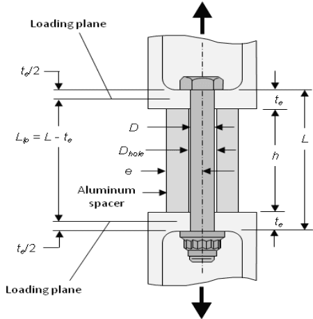
Figure description:
Entities:
- Bolt/Fastener: Central vertical component with a hexagonal head and nut/washers at the bottom.
- Aluminum spacer: Cylindrical sleeve surrounding the bolt shank.
- Loading planes: Two horizontal lines indicating where external tensile force is applied.
- Tensile Load: Represented by black arrows pointing away from the joint at the top and bottom.
Parameters and Dimensions:
- : Total length of the joint/bolt assembly between bearing surfaces.
- : Distance between loading planes, defined as .
- : Height of the aluminum spacer.
- : Thickness of the clamped members; also shown as increments relative to loading planes.
- : Diameter of the bolt shank.
- : Diameter of the hole in the spacer.
- : External diameter or thickness of the aluminum spacer.
Figure 10—Preloaded Joint in which the Bolt Load Increases by a Relatively High Percentage of Applied Tensile Load
Nonlinear finite element analysis of the joint illustrated in Figure 10—with Ec = Eb /3, e/D = 1.5, and n = Llp / L = 0.9—shows that n 0.25.
The conclusion is that, for any practical design with Ec < Eb /3, e/D ≥ 1.5, and n ≤ 0.9, the bolt load increases by no more than 25 percent of the applied tensile load prior to separation.
As shown in Figure 11, Separation before Rupture for a Brittle Threaded Fastening System, when the bolt load increases by 25 percent of the applied tensile load, the joint would separate prior to rupture as long as the preload is not greater than 75 percent of the bolt’s ultimate tensile strength. This is the case even if the fastening system exhibits perfectly brittle failure.
Fastening-system hardware made of metal alloys exhibits some degree of ductility prior to rupture. Ductility causes a joint to separate at a lower applied load than would be predicted with linear theory. Consider a joint in which the bolt load increases by 25 percent of the applied tensile load when linear elastic, with preload at 85 percent of the bolt’s ultimate tensile strength. For such a joint, separation would occur prior to rupture if the plastic deformation, δp , were at least 13.3 percent of the elastic deformation, δe , as shown in Figure 12, Separation before Rupture for a Ductile Threaded Fastening System.
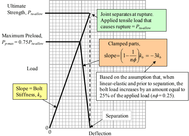
Figure description:
Joint Load-Deflection Characteristics Analysis of Bolt and Clamped Part Loads vs. Deflection
Load-Deflection Diagram for a Bolted Joint
Annotations
- Ultimate Strength, (text_label - position: y = )
- Maximum Preload, (text_label - position: y = 0.75 )
- Joint separates at rupture. Applied tensile load that causes rupture = (text_label - position: At (1.0, 1.0 normalized coordinates))
- Slope = Bolt Stiffness, (text_label - position: Along the main bolt load line)
- Clamped parts, slope = (text_label - position: Along the descending clamped part load line))
- Based on the assumption that, when linear-elastic and prior to separation, the bolt load increases by an amount equal to 25% of the applied load (). (text_label - position: Bottom right explanatory box)
- Separation (text_label - position: On the x-axis at normalized deflection 1.0)
- Rupture/Separation alignment (vertical_line - position: x = 1.0 normalized deflection)
| Deflection (Normalized) | Bolt Load () | Clamped Part Load () |
|---|---|---|
| 0.00 | 0.00 | null |
| 0.75 | 0.75 | 0.75 |
| 1.00 | 1.00 | 0.00 |
Notes: The chart uses a background grid where the Ultimate Strength () is at 20 units vertically and the Separation point is at 20 units horizontally. The Maximum Preload and the point of load divergence occur at 15 units (75% of full scale on both axes. This specific case assumes joint separation and bolt rupture coincide due to the assumption.)
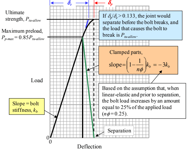
Figure description:
Bolted Joint Load-Deflection Characteristics Analysis of joint separation and bolt failure conditions
Load vs. Deflection Diagram for Bolted Joint
Legend
- Bolt Load curve — color: black; symbol: solid line
- Linear extension of bolt stiffness — color: blue; symbol: solid line
- Clamped parts unloading — color: green; symbol: solid line
- Elastic limit reference — color: black; symbol: dashed vertical line
Annotations
- Slope = bolt stiffness, (text_label - position: Initial linear segment of the bolt load curve)
- Ultimate strength, (horizontal_line - position: y = 100 (top horizontal line))
- Maximum preload, (horizontal_line - position: y = 85 (middle horizontal line))
- Clamped parts, slope = (text_label - position: Adjacent to the green downward-sloping line))
- Separation (text_label - position: x-intercept of the green line)
- If , the joint would separate before the bolt breaks, and the load that causes the bolt to break is . (text_label - position: Top right blue box)
- Based on the assumption that, when linear-elastic and prior to separation, the bolt load increases by an amount equal to 25% of the applied load (). (text_label - position: Lower right white box)
- (text_label - position: Top span from x=0 to vertical dashed line)
- (text_label - position: Top span from vertical dashed line to curve end)
| Deflection (arbitrary units) | Load (arbitrary units) | Component |
|---|---|---|
| 0 | 0 | Bolt (Initial) |
| 17 | 85 | Bolt (Linear Limit / Max Preload) |
| 20 | 100 | Theoretical Linear Bolt Load (end of ) |
| 22 | 100 | Actual Bolt Ultimate Strength (at ) |
| 17 | 85 | Clamped Parts (Start at Preload) |
| 22.7 | 0 | Clamped Parts (Separation point) |
Notes: The diagram illustrates the relationship between bolt load and joint deflection, highlighting key parameters such as ultimate strength, maximum preload, and joint separation conditions based on the ratio of plastic to elastic deflection. The green line represents the decompression of clamped parts starting from the preload state.
Figure 8 states the criterion that to draw the conclusion that a joint would separate before the fastening system ruptures when the maximum preload is no greater than 85 percent of the fastening system's allowable ultimate tensile load. The difference between and (justified in Figure 12) is intentional to account for potential variation in plastic strain between the actual flight hardware and the hardware tested to rupture when determining .
A.6 Ultimate Margin of Safety for Tensile Loading with Linear Theory (Supplement to Section 4.4.1)
Figures 13, Bolt Tensile Load versus Applied Tensile Load; 14, Separation before Rupture with Linear Theory; and 15, Rupture before Separation with Linear Theory, illustrate the linear mechanics of a preloaded joint under applied tensile load in support of section 4.4.1.
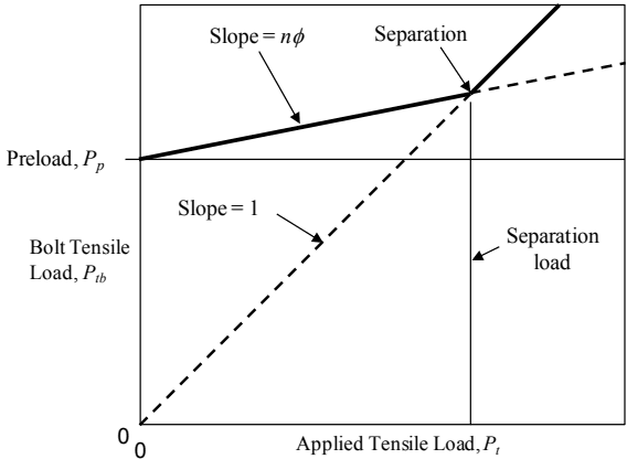
Figure description:
Load Relationship in Bolted Joints
Bolt Tensile Load vs. Applied Tensile Load
Legend
- Bolt Tensile Load behavior — color: black; symbol: Solid line
- Line with Slope = 1 — color: black; symbol: Dashed line
Annotations
- Slope = (text_label - position: On the solid line segment between and Separation load)
- Separation (text_label - position: Intersection point where )
- Slope = 1 (text_label - position: On the dashed line)
- Separation load (vertical_line - position: x-axis value at the separation point)
- Preload, (text_label - position: y-intercept of the solid line)
| Applied Tensile Load, | Bolt Tensile Load, (Solid Line) | Slope = 1 Line (Dashed Line) | Preload Level () |
|---|---|---|---|
| 0 | 0 | ||
| Separation load | Separation load | Separation load | |
| > Separation load |
Notes: The chart illustrates the relationship between bolt tensile load and applied tensile load. Before the 'Separation load' point, the bolt load increases at a slower rate (slope = nϕ starting from the initial preload (Pp. After the separation point, the bolt tensile load increases linearly with a slope of 1, directly following the applied tensile load.))
Figure 13—Bolt Tensile Load versus Applied Tensile Load
Eq. 8 applies until either the bolt ruptures or the joint separates. If the joint separates, the bolt load equals the applied load. (See Figure 13.)
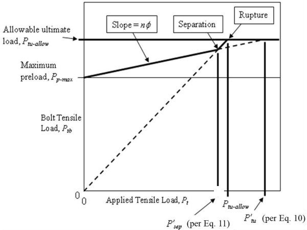
Figure description:
Bolt Tensile Load Diagram
Bolt Tensile Load vs. Applied Tensile Load
Legend
- Bolt Tensile Load, P_{tb} — color: black; symbol: solid line
- Reference Load Path — color: black; symbol: dashed line
- Load Limits — color: black; symbol: thin horizontal lines
Annotations
- Slope = n̴ (text_label - position: on the first segment of the solid bolt load line)
- Separation (text_label - position: at the knee where the solid and dashed lines intersect)
- Rupture (text_label - position: where the solid bolt load line reaches the allowable ultimate load)
- Allowable ultimate load, P_{tu-allow} (text_label - position: y-axis at horizontal limit)
- Maximum preload, P_{p-max} (text_label - position: y-axis at preload horizontal line)
- P'_{sep} (per Eq. 11 (vertical_line - position: x-axis below separation point))
- P_{tu-allow} (vertical_line - position: x-axis below rupture point)
- P'_{tu} (per Eq. 10 (vertical_line - position: x-axis below intersection of dashed line and ultimate load limit))
| Applied Tensile Load () | Bolt Tensile Load () | Line Type | Point Label |
|---|---|---|---|
| 0 | Solid | ||
| (Intersection point) | Solid | Separation | |
| Solid | Rupture | ||
| 0 | 0 | Dashed | |
| (Intersection point) | Dashed | ||
| Dashed | |||
| 0 | Horizontal | Maximum preload level | |
| 0 | Horizontal | Allowable ultimate load level |
Notes: The chart illustrates the behavior of a bolted joint under tensile load. The solid line represents the actual bolt tensile load () starting from an initial preload (). It shows a lower slope (n̴) before separation and a steeper slope (parallel to the dashed line after separation. Rupture occurs when the bolt load reaches the allowable ultimate load limit.)
Figure 14—Separation before Rupture with Linear Theory
If separation would occur before rupture, Eq. 10 does not apply and the margin of safety is given by Eq. 6. (See Figure 14.)
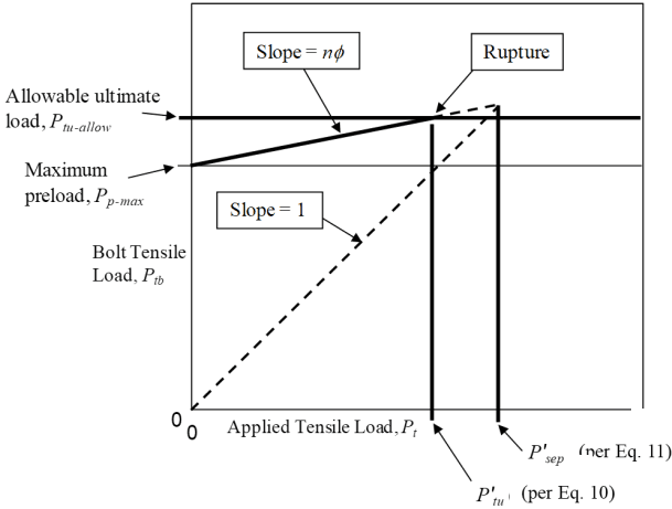
Figure description:
Bolt Tensile Load vs. Applied Tensile Load
Bolt Tensile Load vs. Applied Tensile Load
Legend
- Bolt Tensile Load (Ptb [Solid Line — color: black; symbol: solid line
- Bolt Tensile Load (Ptb [Dashed Line — color: black; symbol: dashed line
- Allowable ultimate load (Ptu-allow — color: black; symbol: thick horizontal line
Annotations
- Slope = nφ (text_label - position: on the solid line starting from Maximum preload)
- Slope = 1 (text_label - position: on the dashed line starting from origin)
- Rupture (text_label - position: at intersection of solid line and Ptu-allow line)
- Allowable ultimate load, Ptu-allow (text_label - position: upper horizontal line label)
- Maximum preload, Pp-max (text_label - position: lower horizontal line starting point label)
- P'tu (per Eq. 10 (vertical_line - position: x = P'tu))
- P'sep (per Eq. 11 (vertical_line - position: x = P'sep))
| Applied Tensile Load () | Bolt Tensile Load () [Solid Line | Bolt Tensile Load () [Dashed Line | Allowable ultimate load () |
|---|---|---|---|
| 0 | 0 | ||
| (Rupture) | |||
| null |
Notes: This is a schematic diagram of bolt load behavior. The bolt tensile load (Ptb initially follows a path with slope nφ starting from the maximum preload (Pp-max. Rupture occurs when the bolt load reaches the allowable ultimate load (Ptu-allow at an applied load of P'tu. The dashed line represents a slope of 1, reaching the separation load P'sep.)))
Figure 15—Rupture before Separation with Linear Theory
If rupture would occur before separation, the margin of safety is given by Eq. 7 (see Figure 15).
A.7 Omission of Preload in Shear and Interaction Analyses (Supplement to Sections 4.4.1 and 4.4.4)
Any fastener loaded in shear should have a full diameter body, and the bolt grip should be selected to ensure the full diameter body is in the shear plane. Specified or allowable shear loads for such fasteners are based on shear tests in which the full diameter body is in the shear plane.
When a preloaded fastener is subjected to shear loading, tensile and shear stresses exist simultaneously in the shank. However, if the shear load is increased until the fastener ruptures, the fastener material first yields and the preload relaxes. As a result, the preload does not contribute to failure.
NASA tests performed in 2009 substantiated the above hypothesis for preloaded fasteners loaded in shear only with no threads in the shear plane. Double-shear specimens with steel plates and A-286 3/8-24 (NAS1956C28) bolts were tested to failure, with the full diameter body in the shear plane. Five bolts were tested without preload and five were tested with preload; all fasteners were from the same procurement lot. Those tested with preload were lubricated with Castrol Braycote® 602EF grease and then torqued to 122 N-m (90 ft-lb), that caused yielding in
the fasteners. Prior to assembly, to minimize friction as a shear-load path, the mating surfaces of the steel plates were lubricated with molybdenum disulfide dry-film lubricant. A fresh set of steel plates was used for each test. The average rupture loads for the two configurations tested showed a difference of less than 2 percent.
Similar results were found in tests of A-286 3/8-24 (NAS1956C14) fasteners under simultaneous tensile and shear loading, conducted in 2010 at MSFC. These tests were performed with and without threads in the shear plane. The tests were performed with and without preload; the tests showed preload had an insignificant effect on the failure loads.
The conclusion from these tests is that preload can be disregarded when assessing ultimate strength for a fastener under shear loading or under simultaneously applied tensile and shear loading.
A.8 Theoretical Treatment of Interaction Equations (Supplement to Section 4.4.4)
The interaction equations for ultimate-strength analysis in section 4.4.4 are based on empirical test data rather than a theoretical derivation. However, similar theoretical interaction equations can be derived when shear, tension, and bending across a cross section are considered. This section presents a classical treatment for interaction of shear, tension, and bending. The equations in this section are not intended to replace the interaction equations in section 4.4.4.
Consider a fastener whose shear plane is in the x-z plane and whose tensile direction is along the z-axis. The fastener is loaded in shear only, developing a shear stress τ. The stress tensor associated with the state of stress is given by
where is used to denote the stress tensor (not to be mistaken with a single stress component ). The principal stresses, given by the eigen values of the stress tensor, are
Using the von Mises yield criterion, one can establish a relationship between the yield stress in tension, Fty , and the yield stress in shear, Fsy . The von Mises criterion is
Using Eqs. 61 and 62 yields
It should be noted that Fsy is not a typically encountered material property. The usual property encountered is the ultimate shear stress Fsu . Often, Eq. 63 is assumed to hold at both yield and ultimate conditions, such that
While Eq. 64 does not have a firm theoretical basis to it, a survey of commonly used materials for fasteners shows that the relationship is typically affirmed.
Now, consider a fastener with a shear and tension at a point in the cross section. The stress tensor for this state of stress is given by
and the principal stresses are given by
Using Eqs. 62, 63, and 66 yields
If Eq. 67 is extrapolated to the ultimate stress condition (which is theoretically incorrect), bending stress is accounted for such that
where is the cross-sectional area; and using , , and , one has
(Eq. 69)
Eq. 69 gives an approximation at the ultimate stress condition for a fastener loaded in shear, bending, and tension in the same cross section.
If the bolt is allowed to yield at ultimate design load, one must accommodate the potential for additional load. For simplicity, the case of combined tension and bending for a circular cross
section with radius r is examined. It is assumed to be an elastic, perfectly plastic material with tensile yield stress of Fty . If a pure axial load is applied such that the entire section has yielded, the fully plastic axial force Np can be computed. Likewise, if the cross section has a pure moment applied such that the upper half is fully yielded to Fty and the lower half is fully yielded to –Fty , the fully plastic moment, Mp , can be computed. These values are computed by the integrals
and
Now consider a section with combined tension and bending at collapse such that the stress distribution is as shown in Figure 16, Stress Distribution at Collapse due to Combined Bending and Tension.
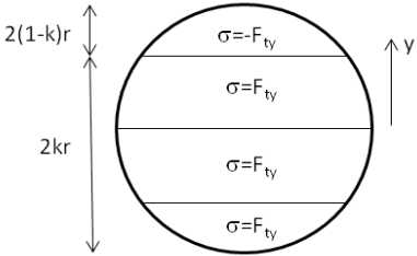
Figure description:
- Shape: A circular cross-section.
- Divisions: Three horizontal lines divide the circle into four horizontal segments.
- Stress Labels:
- Top segment:
- Three lower segments: Each labeled
- Dimensional Indicators:
- Height of the top segment:
- Combined height of the three bottom segments:
- Coordinate System: A vertical arrow on the right labeled "y" pointing upwards.
Figure 16—Stress Distribution at Collapse due to Combined Bending and Tension
One can compute the axial force and moment due to the stress distribution shown in Figure 16 as
and
If either Eq. 72 or Eq. 73 is solved for k, an interaction equation could be written relating the allowable axial load and moment at collapse. The closed-form solution is shown by Eq. 74. (See Stronge & Yu, “Dynamic Models for Structural Plasticity.”)
By comparison, if a rectangular cross section is considered, a simpler expression relating moment and axial load at collapse is found such that
A comparison between Eqs. 74 and 75 is shown in Figure 17, Comparison of Interaction between Circular and Rectangular Cross Sections at Collapse. As can be seen from the figure, there is little difference between the two closed-form solutions. For simplicity, it can be assumed that the interaction equation given by Eq. 75 can be applied to circular cross sections indicative of fasteners.
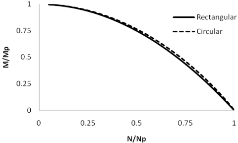
Figure description:
Legend
- Rectangular — color: black; symbol: Solid line
- Circular — color: black; symbol: Dashed line
| N/Np | Rectangular (M/Mp) | Circular (M/Mp) |
|---|---|---|
| 0.00 | 1.00 | 1.00 |
| 0.10 | 0.99 | 0.99 |
| 0.20 | 0.96 | 0.97 |
| 0.30 | 0.91 | 0.93 |
| 0.40 | 0.84 | 0.87 |
| 0.50 | 0.75 | 0.78 |
| 0.60 | 0.64 | 0.68 |
| 0.70 | 0.51 | 0.56 |
| 0.80 | 0.36 | 0.41 |
| 0.90 | 0.19 | 0.23 |
| 1.00 | 0.00 | 0.00 |
Notes: The chart shows the interaction curves for normalized moment (M/Mp versus normalized axial force (N/Np for rectangular and circular cross-sections.))
Figure 17—Comparison of Interaction between Circular and Rectangular Cross Sections at Collapse
To account for shear, a rectangular cross section is used. This simplifies the problem and allows for a simple closed-form solution. For a rectangular cross section, the fully plastic axial force and fully plastic moment are given by
From Eq. 67, the tension-carrying capability of the cross section is reduced due to an applied shear. Eq. 67 can be rewritten in terms of shear Q and fully plastic shear Qp such that
and is the reduced allowable load due to the shear load. Under combined shear, tension, and bending, the peak tensile stress is limited to . Using the same methodology that led to Eqs. 72 and 73, the axial force and moment acting on the cross section due to are
Solving for k and combining Eq. 76 to 78 at collapse yields
Eq. 79 can be simplified and rewritten as
(Eq. 80)
In Eq. 80, the more theoretically appropriate Ftu has been replaced with the term Fbu . It is not uncommon for practitioners to implement a higher allowable based on plastic bending rather than the tensile allowable. Doing so is less conservative, though this approach is accepted due to the conservatism that led to the development of the interaction equation, namely the use of a linear elastic, perfectly plastic material response.
A.9 Determining if Fastener Yielding is Detrimental for Separation or Joint Slip (Supplement to Section 4.4.2)
In a typical joint with preload generated by torque control, fastener yielding under combination of preload and applied load is not detrimental for separation. Rationale:
- a. As shown in Figure 18, Effect of Fastener Yielding on the Separation Load, fastener yielding causes the separation load to be lower than is predicted based on linearly calculated bolt stiffness and clamp stiffness. However, section 4.4.3 requires that the design separation load not exceed minimum preload, which is less than the actual separation load shown in the figure. Thus, fastener yielding that occurs under a given applied load does not affect separation analysis for that load.
- b. Figure 19, Loss of Preload Resulting from Fastener Yielding, shows an example of the loss in preload associated with yielding under an applied load equal to the separation load. Because of strain hardening, reapplication of the same load does not cause further yielding and
the separation load is unchanged. Thus, fastener yielding that occurs under an applied load that does not cause separation is not detrimental for separation under repeated loading.
- c. Figure 20, Fastener Yielding under an Applied Load that Exceeds the Separation Load, shows a situation in which yielding occurs under an applied load that separates the joint. (This situation is possible if the yield factor of safety is greater than the separation factor of safety, in which case the design criteria allow the design yield load to exceed the minimum preload.) Once the applied load is removed, the residual preload is considerably less than the original preload, and the separation load also is below the original preload.
Such yielding can be detrimental for separation if the new separation load is below the minimum preload calculated with Eq. 4. This may be the case if preload is accurately controlled through a method such as ultrasonically measuring the bolt’s change in length. In such a situation, a positive margin of safety for fastener yielding using Eq. 15 ensures the fastener will not yield after separation under the design yield load.
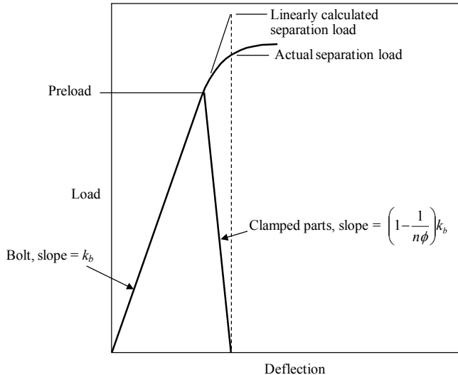
Figure description:
Load vs. Deflection for Bolt and Clamped Parts
Load vs. Deflection Characteristics
Annotations
- Preload (text_label - position: y-axis intercept)
- Linearly calculated separation load (text_label - position: Peak point at deflection for the linear extension)
- Actual separation load (text_label - position: Peak point at deflection for the non-linear curve)
- Bolt, slope = (text_label - position: Initial loading line from origin)
- Clamped parts, slope = (text_label - position: Unloading line from preload to separation point))
- Separation deflection (vertical_line - position: Deflection marked by dashed line)
| Deflection | Bolt (slope ) | Clamped Parts (slope )) | Actual Load Curve | Linear Calc Load Curve |\n| :--- | :--- | :--- | :--- | :--- |\n| 0 | 0 | null | null | null |\n| | Preload | Preload | Preload | Preload |\n| | null | 0 | Actual separation load | Linearly calculated separation load |
Notes: The chart illustrates the load-deflection behavior of a bolted joint from initial preload through to joint separation. It highlights the non-linear nature of the actual separation load compared to a linearly calculated one. and are used to denote deflection at preload and at separation respectively.
Figure 18—Effect of Fastener Yielding on the Separation Load
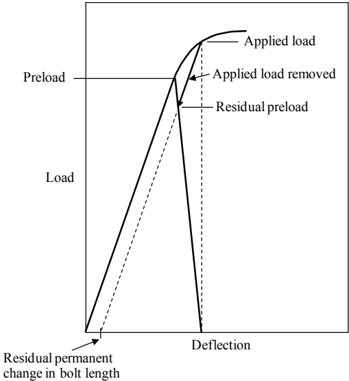
Figure description:
Load-Deflection Diagram for a Bolted Joint
Load vs. Deflection Chart
Annotations
- Preload (text_label - position: y-axis intercept of the initial joint equilibrium point)
- Applied load (text_label - position: Peak of the loading curve)
- Applied load removed (text_label - position: Unloading curve from the peak back towards the residual state)
- Residual preload (text_label - position: Intersection of unloading curve and residual bolt stiffness line)
- Residual permanent change in bolt length (text_label - position: x-axis intercept indicating permanent deformation)
| Feature / State | Deflection | Load | Description |
|---|---|---|---|
| Origin | 0 | 0 | Starting point for bolt deflection |
| Preload | d_p | L_p | Initial assembly state where bolt and member loads balance |
| Applied load | d_max | L_max | Maximum external load applied to the joint, reaching non-linear region |
| Residual preload | d_res | L_res | Preload remaining in the joint after the external load is removed |
| Residual permanent change in bolt length | d_perm | 0 | Permanent set/deformation in the bolt along the deflection axis |
Notes: The chart is a qualitative representation of bolted joint mechanics, showing the relationship between applied load and joint deflection, including the effects of yielding (residual permanent change in bolt length and reduced residual preload. Solid lines represent original loading/unloading paths, while dashed lines indicate the shifted stiffness path after permanent deformation.)
Figure 19—Loss of Preload Resulting from Fastener Yielding
With torque control, there is a wide range between the maximum and minimum preloads calculated per section 4.3.1. Section 4.4.3 specifies a criterion that the design separation load not exceed the calculated minimum preload. If this criterion is satisfied, the design yield load, using typical yield factors of safety for flight hardware, would not exceed the maximum preload and would not cause separation. This premise can be verified by calculation of a yield margin of safety using Eq. 15, if desired.
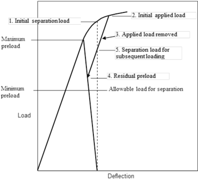
Figure description:
Load-Deflection Characteristics
Load vs. Deflection Curve with Preload and Separation Characteristics
Annotations
- 1. Initial separation load (point - position: Point on the curve where the initial loading path begins to deviate towards the peak)
- 2. Initial applied load (point - position: The maximum load point on the initial loading curve)
- 3. Applied load removed (text_label - position: Points to the unloading curve between point 2 and point 4)
- 4. Residual preload (point - position: The point at which the unloading path ends and the subsequent loading path begins)
- 5. Separation load for subsequent loading (point - position: A point on the subsequent loading curve originating from point 4)
- Maximum preload (vertical_line - position: y = Maximum preload level)
- Minimum preload (vertical_line - position: y = Minimum preload level)
- Allowable load for separation (vertical_line - position: y = Allowable load for separation level)
| Point / Feature | Deflection (Relative Scale) | Load (Relative Scale) |
|---|---|---|
| Origin | 0.0 | 0.0 |
| Minimum preload level | - | 0.25 |
| Allowable load for separation level | - | 0.30 |
| Residual preload (Point 4) | 0.40 | 0.45 |
| Maximum preload level | - | 0.70 |
| Separation load for subsequent loading (Point 5) | 0.45 | 0.65 |
| Initial separation load (Point 1) | 0.50 | 0.85 |
| Initial applied load (Point 2) | 0.55 | 0.90 |
Notes: The chart illustrates the mechanical behavior of a joint or fastener under loading, showing initial loading, unloading, and subsequent reloading paths. It highlights critical parameters such as separation loads and preload levels.
Figure 20—Fastener Yielding under an Applied Load that Exceeds the Separation Load
A possible exception to the above conclusions arises if preload changes significantly under temperature extremes. For example, if preload increases with temperature and yielding occurs at the maximum design temperature, and then the joint later reaches its minimum design temperature, the residual preload may be inadequate to prevent separation under the co-existing design separation load. A recommended criterion for avoiding this situation is to ensure the maximum preload calculated with Eq. 3 does not exceed the fastener’s allowable yield tensile load.
The guidance for determining whether fastener yielding is detrimental for separation also applies to the issue of whether fastener yielding is detrimental for joint slip. In addition, consideration must be given to the situation in which the fastener yields under one loading event such as ground test or liftoff, followed by the design yield shear load in a later event such as maximum air loads during launch. When relying on friction for an alignment-critical joint, it may be wise to assume fastener yielding is detrimental and satisfy the criteria given in section 4.4.2.
A.10 Margin of Safety for Joint Slip (Supplement to Sections 4.4.1 and 4.4.6)
To be consistent with separation analysis (see Appendix A.11), slip analysis is based on the assumption that the clamp force in a preloaded joint is reduced by 100 percent of the applied tensile load. When a joint is concentrically loaded with shear (load passes through bolt-pattern
centroid) and simultaneously loaded in tension, using fasteners of the same type and with the same nominal preload, the friction load, Pf , that can be developed is
where Pt -joint is the total applied tensile load acting on the joint.
Calculation of a margin of safety for slip—that must account for minimum preload, limit loads, and a factor of safety—is not straightforward in such a case. Based on the assumption that, if the applied tensile and shear loads were to increase, they would do so proportionally; one can solve for the proportionality constant, a, that causes a zero-margin condition
where is the coefficient of friction, FS is the appropriate factor of safety for the failure mode affected by slip, PsL-joint is the total limit shear load acting on the joint, and PtL-joint is the total limit tensile load acting on the joint. Solving for a gives
Because a is the scaling factor applied to the external loads that causes a zero-margin condition, the margin of safety for slip is
When no external tensile load is applied, Eq. 84 reduces to
Eqs. 84 and 85 only apply to a joint that is concentrically loaded in tension and shear, has equal nominal preload for all fasteners, and equivalent fastener sizes. When any of these conditions are violated, these equations cannot be used; and an analysis considering these effects must be performed. An example when Eqs. 84 and 85 would not apply is eccentrically loaded joint where the shear produces a resultant torque about the bolt-pattern centroid. A finite element analysis or test can be used to verify that the joint does not slip under such a condition. Another acceptable approach is to assess slip individually at each fastener location as follows:
where PsL is the limit shear load for the fastener and PtL is the limit tensile load for the fastener. Note that, with this approach, a non-negative margin of safety for slip must be shown for each fastener, given that the limit shear and tensile loads may not peak on the same fastener.
A.11 Margin of Safety for Bolted Joint Separation (Supplement to Section 4.4.3)
The numerator in Eq. 19 is Pp-min . Although a bolted joint can withstand an applied tensile load somewhat higher than the preload before separation occurs, it is difficult to conservatively calculate the true separation load. This is true because most methods of analysis used to calculate load sharing in a preloaded bolted joint using bolt stiffness, clamped-material stiffness, and loading-plane factor have been derived from test data with the intention of conservatively predicting the total bolt load. Any such method that conservatively predicts bolt load over- predicts the separation load. In addition, if a preloaded bolt begins to yield under applied tensile load, separation occurs at a lower applied load than linear theory predicts.
In recognition of the above considerations, it was decided that the separation load should be set equal to minimum preload.
A.12 Load Redistribution within a Fastened Joint
When analysis is used to assess the structural integrity of an individual fastener or a group of fasteners in a fastened joint, considerations should be made for the potential of loads to redistribute either due to geometric design features or failure modes. In this section, the following examples are used to illustrate the potential for load redistribution:
- Geometric: Excessive radial clearance between the fastener and clearance hole-bearing surface.
- Localized yielding: Design of yield critical joints compared to bearing critical joints.
- Separation: Changing load paths or mechanical response due to separation.
- Slipping: Distribution of clamp force in the group of fasteners.
A.12.1 Load Redistribution Due to Geometric Features
As an example of load redistribution due to geometric features, a simple lug that is attached by four fasteners is examined, as shown in Figure 21a, Lug with Clearance Holes Example. The fasteners have some amount of radial clearance when situated into the attachment holes of the lug, and the fasteners are not located in the same position relative to the holes. A load is applied such that there are in-plane components of shear and a torque about the bolt pattern centroid. If the lug slips relative to the fasteners, it is likely that the load will redistribute; and the redistribution will be a function of the clearance between the fastener and part, the ductility of each component, and the direction and magnitude of the applied load. For the example shown in Figure 21a, a plausible deformed configuration is shown in Figure 21b, Rigid Body Response for Lug with Clearance Holes, where at most three of the four fasteners may be loaded.
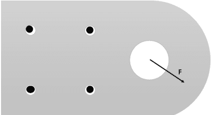
Figure description:
- Grey Component: A lug with a rounded right end.
- Fasteners: Four black circles positioned within larger circular holes in a rectangular pattern on the left side.
- Clearance: Visible white gaps between the black fasteners and the hole edges, showing non-centered placement.
- Large Hole: A single large white circular opening on the rounded end.
- Force Vector: An arrow labeled "F" originates from the center of the large hole, pointing diagonally downward and to the right.
Figure 21a—Lug with Clearance Holes Example
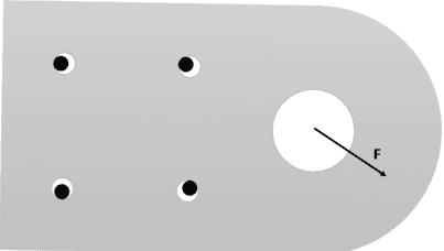
Figure description:
Key Information:
-
Entities:
- Lug: A grey structural component with a rounded end.
- Fasteners/Pins: Four black circular elements positioned in a rectangular pattern on the left side.
- Clearance Holes: White circular regions surrounding the black fasteners, showing offsets (radial clearance.
- Main Hole: A large white circular opening on the right side of the lug.
- Force (F: Represented by a black arrow originating from the center of the large hole, pointing downwards and to the right.
-
Observed Details:
- The four small fasteners are not centered within their respective clearance holes.
- The top-left, top-right, and bottom-right fasteners appear to be in contact with the edges of their holes.
- The bottom-left fastener is centered or near-centered with significant visible clearance around it.
- The force vector F indicates an applied diagonal load.
Figure 21b—Rigid Body Response for Lug with Clearance Holes
For connections that are expected to react shear, to minimize the ramifications of load redistribution, reducing the radial clearances between the hole and fastener surfaces is recommended. If this cannot be accomplished, it should be considered non-conservative to assume the load is equally shared between fasteners. Testing or additional analysis should conservatively bound the expected response of the design.
A.12.2 Load Redistribution Due to Localized Yielding
For the lug shown in Figure 21a, it was hypothesized that potentially only three of four fasteners may be loaded due to the clearance. If the lug is designed to be bearing critical such that the lug material yields before shear failure of the fasteners, some local yielding at a fastener location can cause a redistribution in load. If there is excessive yielding for the example shown in Figure 21a, eventually all fasteners in the pattern may react the forces applied to the lug. However, excessive yielding at a location can have the negative consequence of greater-than-anticipated reactions at other fastener locations. As an example, consider the simple geometry of Figure 22a, Simplified Two-Bolt Plasticity Model, where a component is loaded with some force and reacted at two locations. The bolt-to-component interface is modeled as a spring attached to ground. It is assumed that the bolt closer to the applied force will initially react a greater percentage of the load, and the spring constant k1 is assumed to be 50 percent greater than k2 , and both springs are assumed to have a bilinear force-displacement response such that at a prescribed force magnitude, no additional load is reacted, as shown in Figure 22b, Assumed Plasticity Model.
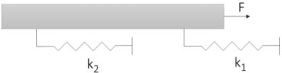
Figure description:
- Horizontal grey bar: Represents a component or structure.
- Applied Force (F: A vector arrow pointing to the right, applied at the end of the bar.
- Springs: Two zigzag lines attached to the underside of the bar and fixed to ground.
- Spring k1: Located closer to the applied force.
- Spring k2: Located further from the applied force.
- Grounding: Vertical lines with hash marks indicating the fixed ends of both springs.
Figure 22a—Simplified Two-Bolt Plasticity Model
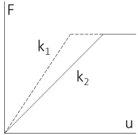
Figure description:
Legend
- k1 — symbol: Dashed line
- k2 — symbol: Solid line
Annotations
- F (text_label - position: Vertical axis label)
- u (text_label - position: Horizontal axis label)
- k1 (text_label - position: Near the dashed line segment)
- k2 (text_label - position: Near the solid line segment)
| Displacement (u) | Force F (k1: dashed line) | Force F (k2: solid line) |
|---|---|---|
| 0 | 0 | 0 |
| u_yield_k1 | F_plateau | F_intermediate |
| u_yield_k2 | F_plateau | F_plateau |
| u_max | F_plateau | F_plateau |
Notes: The graph displays a force-displacement relationship for two systems with different initial stiffnesses, k1 and k2. Both curves follow a linear elastic path starting from the origin (0,0 before reaching a perfectly plastic plateau at the same force level (F_plateau. The dashed line k1 represents a higher stiffness, reaching the yield point at a smaller displacement (u_yield_k1 compared to the solid line k2 which reaches yield at a larger displacement (u_yield_k2.))))
Figure 22b—Assumed Plasticity Model
When this model is loaded, the system response will differ from the elastic solution when the nonlinear response is considered. Figure 23, Difference in Response between Elastic and Elastic- Plastic Model, shows a representative system response, where for a given load, the displacement may be severely under-predicted if the elastic-plastic behavior is not implemented. If this were an alignment critical design, not accounting for the effects of localized yielding could lead to functional performance issues.
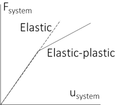
Figure description:
Legend
- Elastic — symbol: Dashed line
- Elastic-plastic — symbol: Solid line
| Elastic-plastic () | Elastic () | |
|---|---|---|
| 0.0 | 0.0 | 0.0 |
| 1.0 | 1.0 | 1.0 |
| 2.0 | 1.4 | 2.0 |
| 3.0 | 1.8 | 3.0 |
Notes: The chart is a conceptual representation of force () versus displacement (). It depicts an initial linear elastic region shared by both models. After a certain displacement, the 'Elastic' model continues linearly as a dashed line, while the 'Elastic-plastic' model (solid line exhibits a reduced slope, representing plastic yielding.)
Figure 23—Difference in Response between Elastic and Elastic-Plastic Model
A.12.3 Load Redistribution Due to Separation
When separation is considered, there is load redistribution similar to when plastic effects are considered. However, in this case when separation occurs, the slope of the applied load and bolt tensile load curve changes such that additional applied tensile load is directly additive to the bolt load, as demonstrated in Appendix A.6.
To demonstrate the effects of separation, a simple two-joint system is considered, as shown in Figure 24, Two-Joint Separation Model. A shear load is applied some distance above the bolted interface plane such that a global heel-toe reaction is envisioned. The fitting on the left side will be loaded in tension whereas the right-side fitting is in compression. The load is transferred to the fittings assuming an infinitely rigid connection. The bolts are considered to be steel, whereas the fitting members are aluminum. For simplicity, the bolts are assumed to have a solid body with a diameter of d = 0.25 in and a head and nut diameter of d = 0.50 in, and each aluminum member is 0.50 in thick and has a 0.001-in radial clearance to the bolt body. In this example, the bolts are assumed to be preloaded to Fpre = 3135 lb, with the exception of the first bolt on the left side that is assumed to be preloaded only to Fpre = 2090 lb.
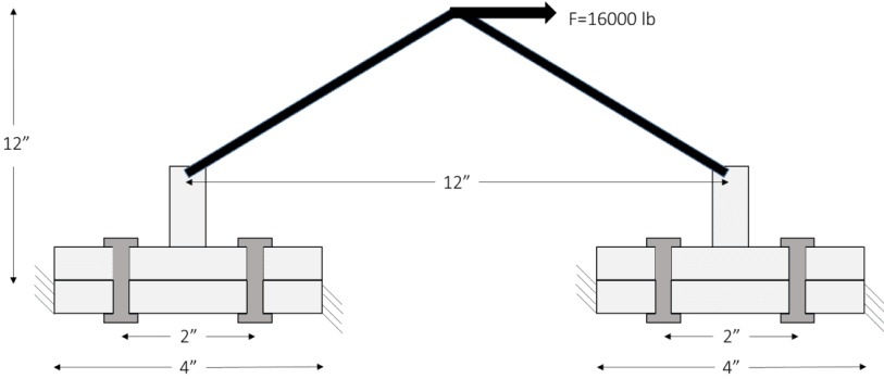
Figure description:
Key Entities and Dimensions:
- Applied Load (F: 16,000 lb, acting horizontally to the right at the apex of the structure.
- Vertical Height: 12" from the base interface to the point of load application.
- Horizontal Distance between vertical members: 12" center-to-center.
- Base Fitting Width: 4" for both the left and right fittings.
- Bolt Spacing: 2" between the two bolts on each fitting.
- Components: Two horizontal joint assemblies, each secured by two bolts, connected by a triangular frame structure. The outer edges of the base plates feature diagonal hatching indicative of fixed supports.
Using the frustum method with a cone angle of 25 degrees to determine the joint stiffness yields a stiffness ratio of = 0.314 for the joint geometry. Also, it is assumed that the load-introduction factor is equal to n = 0.5. With a preload of Fpre = 2090 lb, the interface at the first bolt would be expected to separate locally at approximately
If we assume that both bolts on the left fitting separate at this load (or that both are preloaded to Fpre = 2090 lb), a globally applied load of F = 4958 lb would be calculated to cause separation of the left fitting. However, if we assume that the left fitting will separate based on the total preload of Fpre = 2090 lb for one bolt and Fpre = 3135 lb for the other bolt, the left joint would be expected to be fully separated at a load of
that leads to a globally applied load of F = 6198 lb.
The joint picture above was analyzed using a finite element model that includes touching contact between the bolt and joint members. All contact pairs are assumed to be frictionless. Figure 25, Bolt Forces during Loading of Two-Joint Separation Model, shows individual bolt forces as a function of the externally applied load. The analysis results suggest that partial separation begins below 4300 lb, and full separation of the local region near the first bolt occurs at around 5100 lb. As the first bolt begins to separate, the load redistributes somewhat and the bolt second from the left experiences a slight increase in load. Upon full separation of the first bolt, the load in the second bolt increases more until it too is fully gapped at an external load below the 6198 lb prediction from hand analysis.
The load redistribution within this example has the effect of modifying the system stiffness. The system response is shown in Figure 26, System Stiffness due to Separation and Yielding, in which a baseline analysis assuming no separation is compared to the case where separation can occur. Additionally, a comparison is made to a model that implements typical elastic-plastic behavior for the aluminum and steel members. All models converge to similar response at low load; but when separation occurs, there is a clear change in stiffness. Such effects should be assessed in the design to verify that the functional requirements, both structural and non- structural, are being met. For example, with this example, the change in stiffness could affect the vibrational response of a structure.
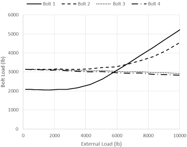
Figure description:
Bolt Load vs. External Load
Legend
- Bolt 1 — color: black; symbol: Solid line
- Bolt 2 — color: black; symbol: Dashed line
- Bolt 3 — color: black; symbol: Dotted line
- Bolt 4 — color: black; symbol: Dash-dot line
| External Load (lb) | Bolt 1 (lb) | Bolt 2 (lb) | Bolt 3 (lb) | Bolt 4 (lb) |
|---|---|---|---|---|
| 0 | 2100 | 3150 | 3150 | 3150 |
| 1000 | 2080 | 3150 | 3130 | 3130 |
| 2000 | 2080 | 3150 | 3100 | 3100 |
| 3000 | 2100 | 3150 | 3100 | 3100 |
| 4000 | 2300 | 3150 | 3050 | 3020 |
| 5000 | 2600 | 3220 | 3050 | 3020 |
| 6000 | 3150 | 3350 | 3020 | 2950 |
| 7000 | 3650 | 3550 | 3020 | 2950 |
| 8000 | 4150 | 3820 | 3000 | 2920 |
| 9000 | 4700 | 4150 | 2980 | 2880 |
| 10000 | 5250 | 4550 | 2920 | 2850 |
Figure 25—Bolt Forces during Loading of Two-Joint Separation Model
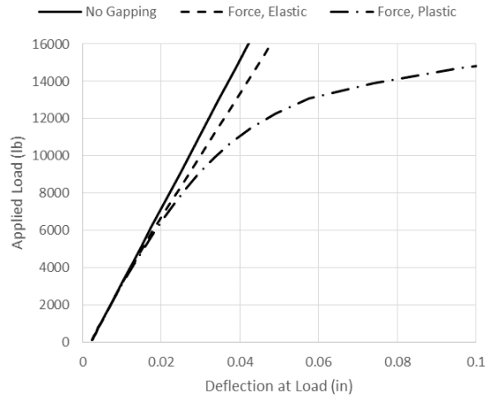
Figure description:
Applied Load vs. Deflection at Load
Applied Load vs. Deflection at Load
Legend
- No Gapping — color: black; symbol: Solid line
- Force, Elastic — color: black; symbol: Dashed line
- Force, Plastic — color: black; symbol: Dash-dot line
| Deflection at Load (in) | No Gapping (lb) | Force, Elastic (lb) | Force, Plastic (lb) |
|---|---|---|---|
| 0.002 | 100 | 100 | 100 |
| 0.01 | 3800 | 3800 | 3800 |
| 0.015 | 5700 | 5400 | 5200 |
| 0.02 | 7600 | 7000 | 6600 |
| 0.03 | 11400 | 10000 | 8800 |
| 0.04 | 15200 | 13200 | 11000 |
| 0.042 | 16000 | null | null |
| 0.047 | null | 16000 | null |
| 0.05 | null | null | 12400 |
| 0.06 | null | null | 13200 |
| 0.07 | null | null | 13800 |
| 0.08 | null | null | 14200 |
| 0.09 | null | null | 14500 |
| 0.1 | null | null | 14800 |
Figure 26—System Stiffness Due to Separation and Yielding
A.12.4 Load Redistribution Due to Slipping
The scenarios described above can act together to cause sufficient load redistribution such that a bolted joint will slip at a load less than predicted. If we consider the case of the two-joint separation model shown in Figure 24 and assume a coefficient of friction of 0.10 between all surfaces, an estimate for the load at which slippage occurs can be determined. A nonlinear finite element model is used to estimate the shear forces acting on each bolt as a function of externally applied shear. Figure 27, Shear Load Acting on Bolt from Slip Analysis, shows that the outer bolts slip first and react the externally applied shear load. It is not until a higher external load that the other fasteners react shear load.
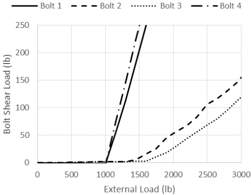
Figure description:
Bolt Shear Load vs External Load
Legend
- Bolt 1 — color: black; symbol: Solid line
- Bolt 2 — color: black; symbol: Long dashed line
- Bolt 3 — color: black; symbol: Dotted line
- Bolt 4 — color: black; symbol: Dash-dot line
| External Load (lb) | Bolt 1 | Bolt 2 | Bolt 3 | Bolt 4 |
|---|---|---|---|---|
| 0 | 0 | 0 | 0 | 0 |
| 250 | 0 | 0 | 0 | 0 |
| 500 | 0 | 0 | 0 | 0 |
| 750 | 0 | 0 | 0 | 0 |
| 1000 | 0 | 2 | 1 | 0 |
| 1250 | 100 | 3 | 2 | 125 |
| 1500 | 200 | 10 | 3 | 250 |
| 1750 | null | 28 | 12 | null |
| 2000 | null | 52 | 22 | null |
| 2250 | null | 78 | 42 | null |
| 2500 | null | 108 | 68 | null |
| 2750 | null | 126 | 92 | null |
| 3000 | null | 155 | 118 | null |
Figure 27—Shear Load Acting on Bolt from Slip Analysis
Figure 28, Contact Status at the Faying Surface during Slip, shows the predicted regions of contact at the faying surface for the two halves of the joint, where a light gray color indicates compressive contact. At initial preload conditions, the compression at the faying surface is consistent except for the left-most fastener location (due to lower preload). Initial slipping occurs at approximately F=1000 lb, where the compression region on the left half of the joint has diminished. After the second slip load near F=1500 lb and beyond, the contact conditions change significantly.
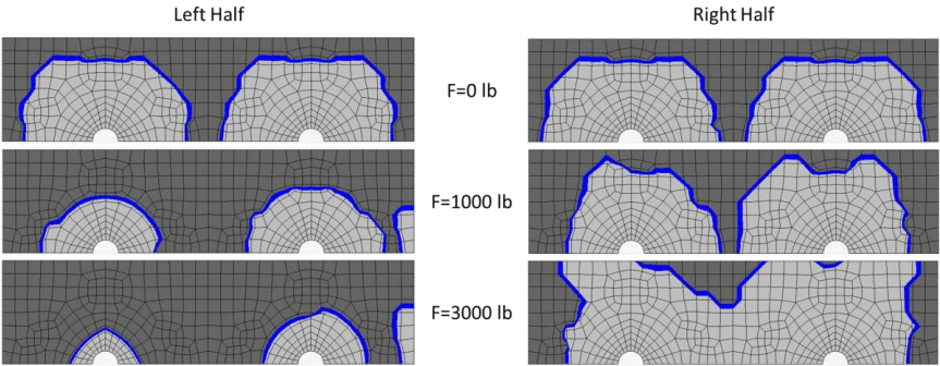
Figure description:
- Headers: Left Half, Right Half.
- Force Values (Rows: F=0 lb, F=1000 lb, F=3000 lb.
- Key Entities:
- Finite Element Mesh: Grid overlaying the entire surface.
- Light Gray Zones: Contact areas centered around circular cutouts.
- Dark Gray Zones: Non-contact or slip areas.
- Blue Borders: Lines defining the boundary between contact and non-contact zones.
- Circular Cutouts: White semi-circular voids located at the base of the contact zones.
- Observations:
- F=0 lb: Shows large, discrete contact zones around each hole in both halves.
- F=1000 lb: Contact zones in both halves are smaller than at 0 lb.
- F=3000 lb: In the Left Half, contact zones have significantly diminished. In the Right Half, contact zones have expanded and merged together.
Figure 28—Contact Status at the Faying Surface during Slip